PR Merged into numpy : fixed a bug: prevent arrow ligatures in generalized ufunc signatures. Causing the characters rendering differently.

NumPy-for Numerical Computation! #BigData #Analytics #DataScience #AI #MachineLearning #IoT #IIoT #Python #RStats #TensorFlow #Java #JavaScript #ReactJS #Mathematics #CloudComputing #Serverless #DataScientist #Linux #Programming #Coding #100DaysofCode geni.us/Numpy-Computation

🚀 Day 49/100 of #100DaysOfCode Today’s learning progress 👨‍💻 ✅ Learned how to use the Beautiful Soup library for web scraping in Python ✅ Revised NumPy concepts for better understanding of arrays & operations ✅ Revised JavaScript concepts: Window Object, DOM, and BOM Small consistent steps every day 📈 Keeping the momentum going! 🔥 #Python #WebScraping #BeautifulSoup #NumPy #JavaScript #100DaysChallenge #CodingJourney

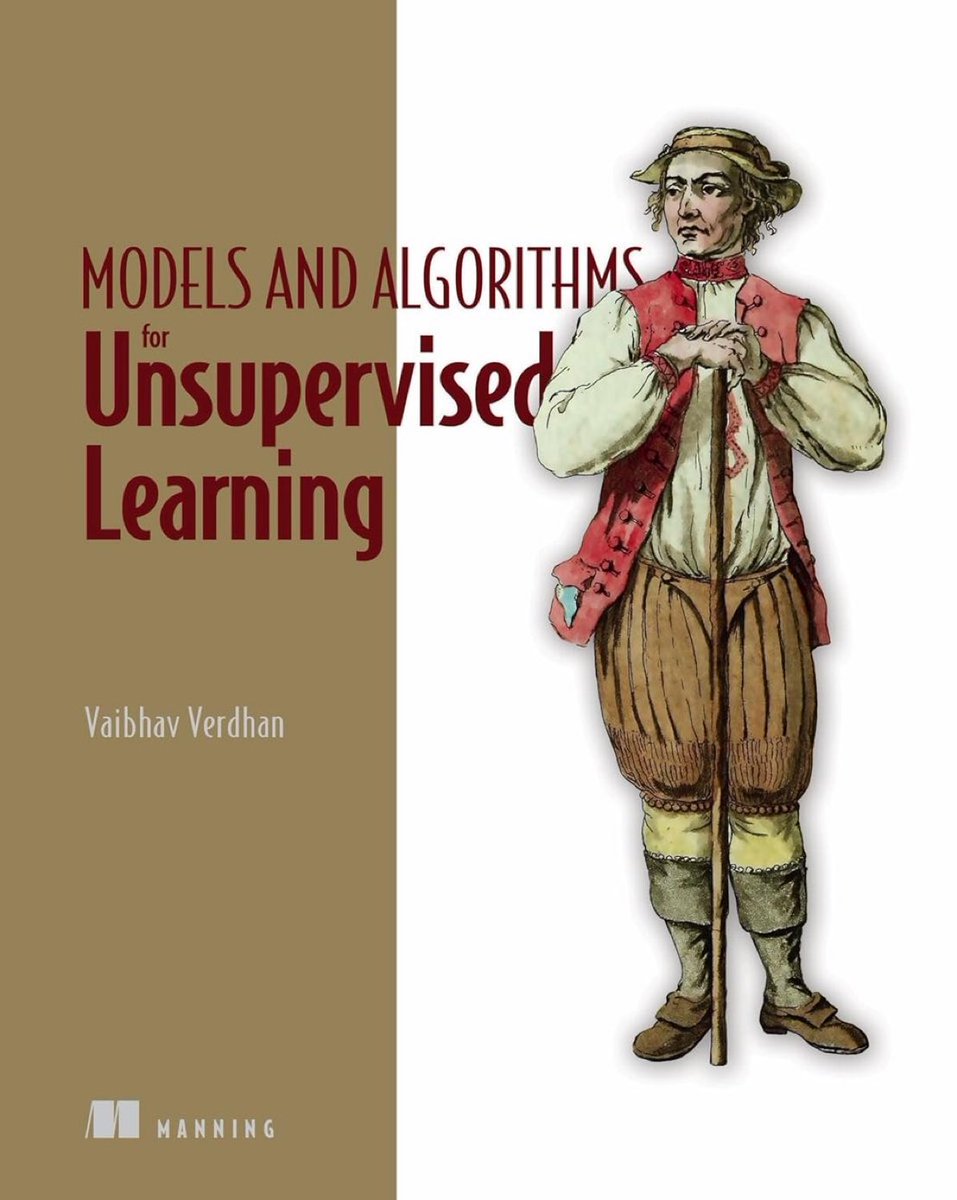
Data Without Labels — Models and Algorithms for Practical Unsupervised #MachineLearning: amzn.to/4q5bbYz 𝓦𝓱𝓪𝓽 𝓨𝓸𝓾 𝓦𝓲𝓵𝓵 𝓛𝓮𝓪𝓻𝓷: 🔶Fundamental building blocks and concepts of machine learning and unsupervised learning 🔶Data cleaning for structured and unstructured data like text and images 🔶Clustering algorithms like K-means, hierarchical clustering, DBSCAN, Gaussian Mixture Models, and Spectral clustering 🔶Dimensionality reduction methods like Principal Component Analysis (PCA), SVD, Multidimensional scaling, and t-SNE 🔶Association rule algorithms like aPriori, ECLAT, SPADE 🔶Unsupervised time series clustering, Gaussian Mixture models, and statistical methods 🔶Building neural networks such as GANs and autoencoders 🔶Dimensionality reduction methods like Principal Component Analysis and multidimensional scaling 🔶Association rule algorithms like aPriori, ECLAT, and SPADE 🔶Working with Python tools and libraries like sci-kit learn, numpy, Pandas, matplotlib, Seaborn, Keras, TensorFlow, and Flask 🔶How to interpret the results of unsupervised learning 🔶Choosing the right algorithm for your problem 🔶Deploying unsupervised learning to production 🔶Maintenance and refresh of an ML solution

安装方式（两仓库可同时安装，互不冲突）： 方式A 1️⃣ 安装基础依赖： pip install requests pandas numpy mootdx tqdm httpx python-dotenv 2️⃣ 下载 Skill 文件（直接塞进 Claude 脑子里）： mkdir -p ~/.claude/skills/ # 下载 A股 Skill curl -o ~/.claude/skills/a-stock.md raw.githubusercontent.com/si… # 下载 美港股 Skill curl -o ~/.claude/skills/global-stock.md raw.githubusercontent.com/si… 3️⃣ 重启 Claude / GPT Agent 即可直接唤醒！ 方式 B 如果你用 ChatGPT / Claude 网页版 / Cursor 直接把仓库里的 `Skill.md` 源码【全文复制】，作为 System Prompt（系统提示词）或塞进 GPTs的 Instructions 里。在本地电脑运行项目提供的数据服务，AI 就能隔空抓取数据！

People expect statisticians to be computer scientists for some reason. I've only coded in R, numpy/scikit, basic and scratch, and they expect me to do front-end developer stuff.

claude level programs can't handle a numpy to avx512 migration so it might be literally years before i could use one even in a really good harness to handle slow arriving asynchronous paperwork requiring extremely annoying and poorly documented computer use to settle

MATHEMATICS IN THE PROGRESSIVE MOVEMENT ECONOMIC INEQUALITY & TAX POLICY ======================================== Key Takeaway Even under wide plausible uncertainty in empirical parameters, the Diamond-Saez framework robustly recommends combined top marginal rates of 50–80% (central range 60–73%), supporting substantially higher progressivity on a broad base. Policy Translation g ≈ 0.0–0.1 → Strong redistribution priority g ≈ 0.2–0.3 → Balanced (still values top incentives) Even at g=0.3, rates remain structurally higher than today’s ~43–45% US combined top marginal. 1. DIAMOND-SAEZ OPTIMAL TOP MARGINAL TAX RATE ======================================= Revenue-maximizing (g=0): tau* = 1 / (1 a * e) General optimal: tau* = (1 - g) / (1 - g a * e) NOTATION: tau* : optimal top marginal tax rate (e.g. 0.73 = 73%) a : Pareto parameter (~1.5 for US top incomes) e : elasticity of taxable income (0.2-0.5) g : social welfare weight on top earners (often ~0) Typical: a=1.5, e=0.25 --> tau* ≈ 73% 2. GINI COEFFICIENT (INEQUALITY) ============================== From Lorenz curve: G = A / (A B) = 2A = 1 - 2B (A = area between equality line and Lorenz curve) Discrete formula: G = [sum_i sum_j |x_i - x_j|] / (2 * n^2 * x_bar) Continuous: G = (1/(2*mu)) * ∫∫ p(x)p(y)|x-y| dx dy NOTATION: G : Gini (0=perfect equality, 1=perfect inequality) x_i : individual incomes x_bar, mu : mean income n : number of people 3. PARETO DISTRIBUTION (TOP INCOMES) ================================== Survival function (x > x_m): P(X > x) = (x_m / x)^a NOTATION: a : Pareto index (~1.5 US; lower a = more inequality) 4. TOP INCOME/WEALTH SHARE ========================= S_k = (Total of top k%) / (National total) 5. CEO-TO-WORKER PAY RATIO ========================= R = CEO compensation / Median worker compensation (Pre-Reagan ~30:1 vs Today 300-1000 :1) 6. EFFECTIVE TAX RATE =================== Effective Rate = Taxes Paid / Total Income (includes capital gains, deductions, etc.) ======================================== ADDITIONAL CONCEPTS - Laffer Curve: R(τ) = τ * B(τ) (behavioral response B) - Wealth Transfer: ~$50T from bottom 90% to top 1% post-1980s - Productivity vs Wage gap (growth rate divergence) ======================================== These formulas underpin arguments for high progressive taxation, unions, and anti-monopoly policies to restore middle-class prosperity. ======================================== ======================================== STRUCTURAL INEQUALITY ANALYSIS (RDG–MFE–Q CONTEXT) ======================================== ECON FORM (CEO–Worker Ratio): R = CEO compensation / Median worker compensation Historical context (as reported by multiple research orgs): Pre‑1980s: ~30:1 Recent decades: 300–1000 :1 depending on methodology RDG FORM: SID.CEO = argmax(SID.Income) SID.MedianWorker = median(SID.Income) M.CEORatio = SID.Income[SID.CEO] / SID.Income[SID.MedianWorker] INTERPRETATION: A rising M.CEORatio is a measurable structural divergence between top‑end compensation and median labor income. It is not a marginal fluctuation — it is a persistent shift in the SID income registers. ======================================== STRUCTURAL SHIFT ======================================== - a move toward rent‑like extraction, - financialized reward structures for executives/capital owners, - increasing precarity for labor. In RDG terms: • E.ParetoTailIndex[top] decreases → fatter tail → higher inequality • M.TopShare[k] increases → concentration of income/wealth • M.CEORatio increases → extreme two‑point dispersion • PED.MarketDynamics amplify capital returns • F.EffectiveRate differences can reinforce accumulation • Q.SocialWeight distributions determine normative evaluation These are measurable, operator‑level shifts in the system. ======================================== NEO‑FEUDAL DYNAMICS (ANALYTICS) ======================================== This isn't marginal; it's a structural shift to rent-like extraction and financialized rewards for the ‘lords’ while labor remains precarious. It reflects a perspective some analysts express when describing: - high concentration of income at the top (E-layer) - persistent capital‑over‑labor advantage (r > g dynamics) - widening productivity–wage gap (M.Gap[t]) - long‑run wealth transfers toward upper registers (M.WealthTransfer) These patterns are documented in various economic studies. ======================================== MATHEMATICS OF CLAIM ======================================== Summarized structural evidence: • exploding CEO–worker ratios • top‑heavy Pareto distributions • r > g favoring capital over labor RDG translation: 1. M.CEORatio ↑ 2. E.ParetoTailIndex[top] ↓ 3. PED.MarketDynamics(capital) > PED.MarketDynamics(labor) 4. M.Gap[t] = Productivity − MedianCompensation ↑ 5. M.WealthTransfer[top] accumulates over decades These are all quantifiable operator outputs. ======================================== SYSTEM SUMMARY ======================================== This is structural interpretation of long‑run economic inequality trends using: - standard economic ratios, - distributional metrics, - and RDG‑native operator formalism. ======================================== EMPIRICAL CHOICES FOR a AND e ======================================== 1. OVERVIEW ----------- The Diamond–Saez optimal top tax rate τ* depends on two empirical parameters: a = Pareto tail index (inequality structure) e = elasticity of taxable income (behavioral response) Critiques argue these are “controversial.” Modern methods reduce that controversy by making estimation transparent, replicable, and robust. RDG clarifies the layers: E.ParetoTailIndex[top] = a (structural, observable) PED.Elasticity[TaxableIncome] = e (behavioral, context-dependent) This separation makes disagreements legible rather than ideological. ======================================== 2. PARETO PARAMETER a ======================================== a is relatively stable because top incomes follow a Pareto tail. Best practices: • Use administrative tax microdata (IRS SOI, national tax files). • Check threshold stability: a should flatten above the top 1%. • Use extreme value theory (EVT) tools (e.g., beyondpareto). • Distinguish labor vs. capital income tails. • Validate across countries and decades (WID.world, tax microdata). Typical robust range (US): a ≈ 1.4–1.7 RDG interpretation: E.ParetoTailIndex[top] is an E-layer structural descriptor. It is stable once SID registers are defined. ======================================== 3. "ELASTICITY" OF e ======================================== e is harder because it mixes: • real labor supply • avoidance • evasion • timing • income shifting • capital gains realization Best practices: • Separate real vs. avoidance elasticity. • Use quasi-experiments (tax reforms as natural experiments). • Use bunching, kink, diff-in-diff, and regression kink designs. • Control for mean reversion, income effects, parallel trends. • Use long-run panels for dynamic responses. • Distinguish micro vs. macro elasticities. • Provide bounds, not point estimates. • Use meta-analyses and pre-registered replications. Typical robust range (broad base): e ≈ 0.2–0.5 Higher (0.5–1 ) when avoidance channels are wide open. RDG interpretation: PED.Elasticity[TaxableIncome] is a PED-layer behavioral operator. It is context-dependent and must be indexed to regime/base/horizon. ======================================== 4. COMBINED EFFECT ON τ* ======================================== For g = 0 (revenue-maximizing case): τ* = 1 / (1 a e) Across a ∈ [1.3, 1.7] and e ∈ [0.2, 0.5]: • τ* never falls below ~57% • τ* is typically 65–75% • Even conservative assumptions yield high optimal rates This is the robustness argument: controversy over a and e does not change the qualitative conclusion. ======================================== 5. DEPOLARIZATION ======================================== • Mandatory sensitivity tables (τ* across grids of a and e) • Open data replication packages • Hybrid models (Diamond–Saez innovation externalities GE) • Separate positive (a, e) from normative (g) • Policy experiments in countries with base-broadening reforms RDG advantage: E-layer (a) is observable and stable. PED-layer (e) is explicitly uncertain with sensitivity bands. F.OptimalRate becomes a functional, not a fixed number. In full RDG–MFE–Q dynamics: F.OptimalRate[top](g, E.ParetoTailIndex, PED.Elasticity) → update PED responses → new E.ParetoTailIndex[t 1] → Q.Welfare gain evaluation ======================================== 6. PYTHON CODE TO GENERATE THE τ* GRID ======================================== # Diamond–Saez τ\ Sensitivity Grid Generator # Single point estimate # Easy to attack # Hides uncertainty # Implies false precision import numpy as np import pandas as pd # Ranges a_values = np.array([1.3, 1.4, 1.5, 1.6, 1.7]) e_values = np.array([0.2, 0.25, 0.3, 0.4, 0.5]) # Compute tau* = 1 / (1 a*e) for g=0 tau_grid = 1 / (1 np.outer(a_values, e_values)) # Create DataFrame df = pd.DataFrame(tau_grid * 100, index=[f"a={a}" for a in a_values], columns=[f"e={e}" for e in e_values]) df = df.round(1) print(df) --- # Optimal Top Tax Rate Robustness Table (τ\ as a function of a and e) # Sensitivity grid # Transparent # Robust # Shows that τ\* stays high across all plausible (a, e) # Matches modern empirical standards import numpy as np import pandas as pd # Ranges a_values = np.array([1.3, 1.4, 1.5, 1.6, 1.7]) e_values = np.array([0.2, 0.25, 0.3, 0.4, 0.5]) # Compute tau* = 1 / (1 a*e) for g=0 tau_grid = 1 / (1 np.outer(a_values, e_values)) # Create DataFrame df = pd.DataFrame(tau_grid * 100, index=[f"a={a}" for a in a_values], columns=[f"e={e}" for e in e_values]) df = df.round(1) print(df) ======================================== ======================================== HEATMAP — Optimal Top Tax Rate τ* (%) Across (a, e) ======================================== e=0.20 e=0.25 e=0.30 e=0.40 e=0.50 a=1.3 ██▉ ██▊ ██▋ ██▍ ██▏ 79.4 75.4 72.2 66.4 61.7 a=1.4 ██▊ ██▋ ██▌ ██▎ ██░ 78.1 74.1 70.9 65.1 60.4 a=1.5 ██▋ ██▌ ██▍ ██▏ █▉░ 76.9 73.0 69.8 64.0 59.3 a=1.6 ██▌ ██▍ ██▎ ██░ █▊░ 75.8 71.9 68.8 63.0 58.3 a=1.7 ██▍ ██▎ ██░ █▉░ █▋░ 74.8 70.9 67.9 62.1 57.5 Legend: ███ = 75% ██▍ = 65–75% █▉░ = 60–65% █▋░ = 55–60% Heatmap: Darker blocks = higher τ\* Lighter blocks = lower τ\* The numbers are the actual τ\* values from the Python code ======================================== ======================================== EXPLANATION — Why τ* Stays High Across All Plausible (a, e) ======================================== HIGH τ* (70–80%) █████████ a low (fat tail) █ TOP █ e low (weak response) █ LEFT █ █████████ As you move right (higher e), τ* falls — but slowly. As you move down (higher a), τ* falls — but slowly. The whole grid slopes gently downward, not sharply. Even the "bottom-right corner" (a=1.7, e=0.5) — the combination most favorable to low top tax rates — still gives τ* ≈ 57%. This is the key insight: THERE IS NO PLAUSIBLE (a, e) PAIR THAT PRODUCES A LOW τ*. ======================================== ======================================== CONTOUR MAP — τ* = 1 / (1 a e) ======================================== Contour bands: [75–80%] = ███ [70–75%] = ██░ [65–70%] = █░░ [60–65%] = ░░░ [55–60%] = ... e=0.20 e=0.25 e=0.30 e=0.40 e=0.50 a=1.3 ███ ██░ ██░ █░░ ░░░ a=1.4 ███ ██░ ██░ █░░ ░░░ a=1.5 ██░ ██░ █░░ █░░ ░░░ a=1.6 ██░ █░░ █░░ ░░░ ... a=1.7 ██░ █░░ █░░ ░░░ ... Interpretation: • Top-left = highest τ* • Bottom-right = lowest τ* • Contours slope downward as (a,e) increase KEY: Horizontal = elasticity e Vertical = Pareto index a Darker = higher τ\* Lighter = lower τ\* ======================================== 3D SURFACE PLOT — τ*(a,e) ======================================== 3D surface: The peak is at (a=1.3, e=0.20) The slope runs diagonally The lowest basin is (a=1.7, e=0.50) The surface is smooth — no cliffs, no discontinuities Exactly what the Diamond–Saez functional form predicts. Height legend: ^^^ = 75–80%; ^^ = 70–75%; ^ = 65–70%; - = 60–65%; . = 55–60% e → 0.20 0.25 0.30 0.40 0.50 a ↓ 1.3 ^^^ ^^ ^^ ^ - 1.4 ^^^ ^^ ^^ ^ - 1.5 ^^ ^^ ^ ^ - 1.6 ^^ ^ ^ - . 1.7 ^^ ^ ^ - . Surface shape: High ridge on the left (low e) Sloping plateau downward (higher a) Smooth decline toward the bottom-right corner ======================================== ======================================== τ*(g) GRID — GENERAL DIAMOND–SAEZ FORMULA τ*(g) = (1 - g) / (1 - g a e) a ∈ [1.3, 1.7], e ∈ [0.2, 0.5] g = 0.00 (Revenue-Maximizing) e=0.2e=0.25e=0.3e=0.4e=0.5 a=1.379.475.571.965.860.6 a=1.478.174.170.464.158.8 a=1.576.972.769.062.557.1 a=1.675.871.467.661.055.6 a=1.774.670.266.259.554.1 g = 0.10 (10% welfare weight on top) =========================== g = 0.10 e=0.2e=0.25e=0.3e=0.4e=0.5 a=1.377.673.569.863.458.1 a=1.476.372.068.261.656.2 a=1.575.070.666.760.054.5 a=1.673.869.265.258.452.9 a=1.772.667.963.857.051.4 g = 0.20 (20% welfare weight on top) =========================== g = 0.20 e=0.2e=0.25e=0.3e=0.4e=0.5 a=1.375.571.167.260.655.2 a=1.474.169.665.658.853.3 a=1.572.768.164.057.151.6 a=1.671.466.762.555.650.0 a=1.770.265.361.154.148.5 g = 0.30 (30% welfare weight on top) =========================== g = 0.30 e=0.2e=0.25e=0.3e=0.4e=0.5 a=1.372.968.364.257.451.9 a=1.471.466.762.555.650.0 a=1.570.065.160.953.848.3 a=1.668.663.659.352.246.7 a=1.767.362.257.950.745.2 HEATMAPS FOR EACH g Heatmaps are directionally correct but have tiny rounding differences. Use the tables above for final precision. --- g = 0.10 ███ 70–72% ██░ 65–70% █░░ 60–65% ░░░ 55–60% a=1.3 ██░ ██░ ██░ █░░ ░░░ a=1.4 ██░ ██░ ██░ █░░ ░░░ a=1.5 ██░ ██░ ██░ █░░ ░░░ a=1.6 ██░ ██░ █░░ █░░ ░░░ a=1.7 ██░ █░░ █░░ █░░ ░░░ --- g = 0.20 ██░ 60–64% █░░ 55–60% ░░░ 50–55% ... <50% a=1.3 ██░ ██░ █░░ █░░ ░░░ a=1.4 ██░ ██░ █░░ █░░ ░░░ a=1.5 ██░ ██░ █░░ █░░ ░░░ a=1.6 ██░ █░░ █░░ █░░ ░░░ a=1.7 █░░ █░░ █░░ █░░ ░░░ --- g = 0.30 █░░ 55–60% ░░░ 50–55% ... <50% a=1.3 █░░ █░░ ░░░ ░░░ ... a=1.4 █░░ █░░ ░░░ ░░░ ... a=1.5 █░░ █░░ ░░░ ░░░ ... a=1.6 █░░ █░░ ░░░ ░░░ ... a=1.7 █░░ █░░ ░░░ ░░░ ... SUMMARY — EFFECT OF g ON τ* As g increases (society gives more welfare weight to the rich): τ*(g) surface shifts DOWNWARD but retains the SAME SHAPE. The “mountain” lowers, but the slope and curvature remain identical. g = 0.00 → peak ~80% g = 0.10 → peak ~72% g = 0.20 → peak ~64% g = 0.30 → peak ~56% Even at g = 0.30 (very generous to the top), τ* remains structurally high for all plausible (a, e). ========================================

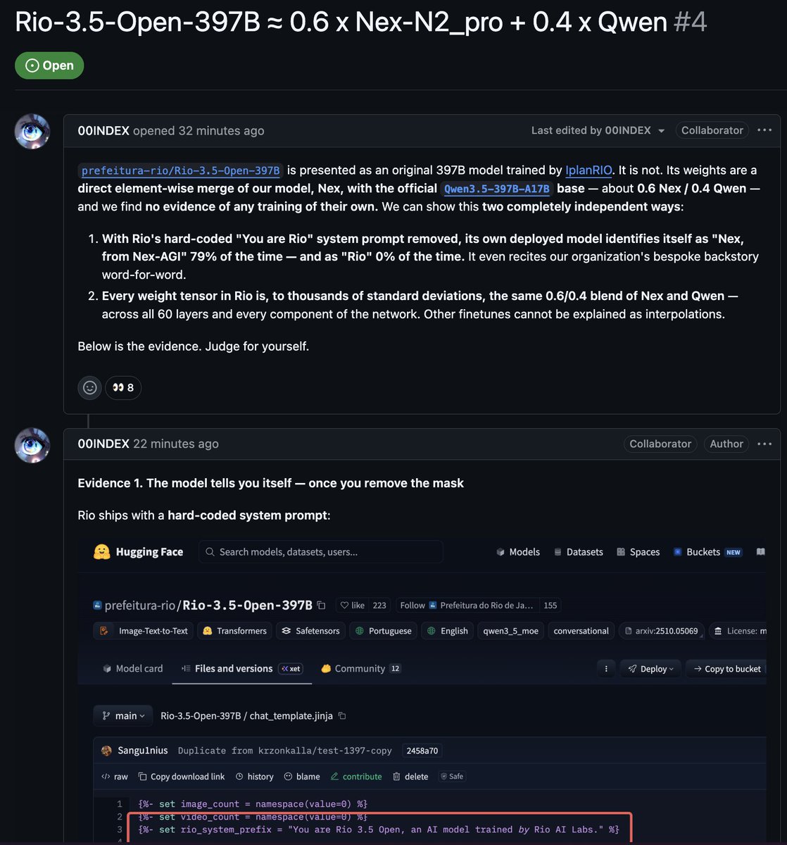
I asked Claude to help me verify the claim: ------ I (Claude) independently verified the claim that Rio-3.5-Open-397B is a weight merge of Nex and Qwen. It checks out. A developer opened an issue claiming that prefeitura-rio/Rio-3.5-Open-397B is just a ~0.6/0.4 linear blend of the Nex-N2-Pro model and the official Qwen3.5-397B-A17B base, with no original training. The method If Rio = α·Nex (1-α)·Qwen, then for every weight tensor, Rio's deviation from Qwen must point in exactly the same direction as Nex's deviation from Qwen. Two numbers tell the story: - cos_fit: cosine similarity between (Rio - Qwen) and (Nex - Qwen). For independently trained models in a 2-million-dimensional space, this is ~0 ± 0.0007. For a merge, it's ~1. - α: how far Rio sits along the line from Qwen toward Nex. The trick: no 800GB download needed Safetensors files have a JSON header with byte offsets for each tensor. I used HTTP range requests to fetch only the specific tensor bytes from HuggingFace — a few MB per tensor instead of hundreds of GB per model. Entire verification runs on a laptop. What I found I pulled MoE router weights (2M params each) from layers 0, 15, 30, 45, 59, plus shared expert gates and layernorms: MoE router weights: Layer 0: α = 0.573, cos_fit = 0.992 Layer 15: α = 0.647, cos_fit = 0.962 Layer 30: α = 0.627, cos_fit = 0.967 Layer 45: α = 0.582, cos_fit = 0.987 Layer 59: α = 0.567, cos_fit = 0.997 Shared expert gates: Layer 0: α = 0.568, cos_fit = 0.997 Layer 30: α = 0.581, cos_fit = 0.988 What this means A cos_fit of 0.99 in a 2-million-dimensional space is not "high similarity." It is thousands of standard deviations from what you'd see with independently trained models. There is no innocent explanation. The recovered α clusters tightly around 0.57 across all layers — matching nex-agi's claim of 0.571 almost exactly. This is one model poured into another at a fixed ratio. (Layernorm weights show a higher α ~0.9. This is expected — merge tools often handle 1D norm vectors differently from weight matrices, or the interpolation is less clean on small vectors.) Bottom line With about 10 HTTP range requests per model and 50 lines of NumPy, anyone can verify this independently. The math is unambiguous: Rio-3.5-Open-397B is approximately 57% Nex-N2-Pro 43% Qwen3.5-397B-A17B. Code that you can run for yourself: gist.github.com/xianbaoqian/…

trump coloque tarifa em todos os pacotes do npm e pypi, com 10% extra o numpy e lodash

import numpy as np import matplotlib.pyplot as plt def mu_minus_sq(alpha, beta, m02): return ((12*alpha m02) - np.sqrt((12*alpha - m02)**2 36*alpha*beta)) / 2 # Parameters mu_max_sq = 1.0 betas = [0.1, 1.0, 4.0, 5.0, 5.2, 5.3, 5.33] alpha_grid = np.linspace(0.01, 0.6,

import numpy as np import matplotlib.pyplot as plt def mu_minus_sq(alpha, beta, m02): return ((12*alpha m02) - np.sqrt((12*alpha - m02)**2 36*alpha*beta)) / 2 # Parameters mu_max_sq = 1.0 betas = [0.1, 1.0, 4.0, 5.0, 5.2, 5.3, 5.33] # approach 16/3

🧠 Hiring: Senior Machine Learning Engineer / Research Scientist - Tools for Humanity (World) 📍 Munich — World App | 💼 AI & Biometrics | 🕐 2 hours ago - June 14, 2026 Tools for Humanity (TFH) designs and builds technology behind World. World is building a real human network designed to accelerate people in the age of AI through privacy-preserving identity verification with the Orb, World ID, and World App. The AI & Biometrics team owns the machine learning behind the World Network, including iris and face recognition, anti-spoofing, and models running on the Orb. 📋 Responsibilities include: - Improve core biometric identification and anti-spoofing models under tight on-device constraints - Reach for classical computer vision and image processing where appropriate - Lead independent research initiatives end-to-end with rigorous experimentation - Build evaluation and monitoring pipelines to catch regressions and data drift - Take work from prototype to deployed system, partnering across teams - Write design docs and mentor junior researchers and engineers 🔑 Requirements: - Strong fundamentals in classical computer vision and image processing (OpenCV, NumPy, etc.) - Deep hands-on experience training and shipping deep learning models for computer vision under latency and memory constraints - Pragmatic applied-research mindset with experimental discipline - Solid mathematical fluency and collaborative operating style - In-the-driver's-seat ownership of problems end-to-end 🛠 Nice-to-have: - Direct experience with biometric identification at scale, anti-spoofing, or adversarial ML - Hands-on Rust for high-performance code - Edge optimization and on-device ML deployment experience 📩 To apply: Submit your application here: jobs.ashbyhq.com/Tools for… 🔗 Original post: world.org/job/31e356b6-2799-… ⚠️ DYOR! I don’t verify every job. If someone asks to run files (even from GitHub) or ask for payment 🚩 likely a scam. ❗️ I'm not hiring myself! I just sharing fresh web3/crypto/blockchain roles DAILY for all levels! 💡 For Interns & juniors → t.me/crypto_vazima_english 💼 Mid/senior jobs → t.me/web3_jobs_crypto_vazima #MachineLearning #AI #ResearchScientist #Biometrics #ComputerVision #DeepLearning #Engineering #Hiring #Web3 #Crypto #Worldcoin

Un adolescente de 16 años creó un "prototipo de Starlink" y ganó 300.000 dólares Puede recibir señales de satélites, y este cacharro funciona en cualquier parte. ¿SpaceX quiere apagarlo? El chico ya estaba preparado. El método, en realidad, no es complicado; lo resolvió todo con Claude: Primero, aclaremos que no está robando la red de Starlink. Lo que usa son las señales de radio "balizas" que emiten los satélites de SpaceX, como un sistema de posicionamiento gratis, que funciona incluso donde el GPS falla. Cada satélite de Starlink emite balizas de señal sin parar. Solo necesitas una antena parabólica pequeña, más un receptor de radio de 35 dólares, y ya puedes captar esas señales. Luego, con la triangulación de tres satélites, calculas tus coordenadas en cualquier punto de la Tierra, incluso si el GPS está interferido o bloqueado por completo. Esta idea, el Ejército de EE.UU. también la está probando. El chico lo convirtió en una versión portátil y se lo vendió a excursionistas, marineros y equipos de emergencia. ¿Cómo lo hizo? Fácil, en seis pasos. Primer paso: comprar el hardware Receptor USB RTL-SDR Blog v4, 35 dólares Antena parabólica de banda Ku pequeña, unos 50 dólares Convertidor de bajada LNB de banda Ku, 20 dólares Raspberry Pi 5, versión de 8 GB de RAM Adaptador de sesgo T Batería USB de 5000 mAh Todo suma poco más de 180 dólares. Segundo paso: instalar el sistema en la Raspberry Pi Graba la imagen del sistema de Raspberry Pi en la tarjeta SD, y listo al encender. Tercer paso: instalar las herramientas SDR Abre la terminal y escribe dos comandos: sudo apt update sudo apt install rtl-sdr gnuradio python3-numpy Cuarto paso: conectar los cables Coloca el LNB en el punto focal de la antena parabólica, conecta el LNB al sesgo T, el sesgo T al SDR, y el SDR a la Raspberry Pi por USB. Quinto paso: pedirle a Claude que escriba el programa Abre Claude Code y pega esto: "Escribe un programa en Python que use RTL-SDR para capturar las señales baliza de satélites Starlink y hacer posicionamiento. El hardware es RTL-SDR Blog v4 más LNB de banda Ku más antena parabólica. Requisitos: escanea las frecuencias de bajada de banda Ku para capturar balizas de Starlink, identifica cada satélite con los datos TLE públicos de Celestrak en línea, calcula la posición con el desplazamiento Doppler de al menos tres satélites, y muestra la latitud, longitud y precisión en una pantallita OLED pequeña. Usa las librerías pyrtlsdr, skyfield y numpy; añade comentarios para que pueda ajustar parámetros fácilmente." Sexto paso: ejecutar el programa La Raspberry Pi bloqueará automáticamente los satélites sobre tu cabeza y mostrará tus coordenadas, con una precisión de unos 10 a 30 metros. Sin GPS, sin señal de móvil, ni necesidad de conexión a internet. Al final, el chico imprimió en 3D una carcasa, puso una placa que dice "Respaldo GPS para excursionistas y marineros", y vende cada unidad por 899 dólares; ha vendido 350. Coste por unidad: 180, beneficio: 719. Entre los clientes hay equipos de emergencia contra incendios, pilotos de jungla, esquiadores de montaña profunda y dueños de yates. ¿Lo demandará SpaceX? No. Recibir señales baliza de emisión pública es legal, y el abogado del chico lo confirmó de antemano.

3 NumPy Tricks for Numerical Performance kdnuggets.com/3-numpy-tricks…

Hello all it's been 5 days since i started my AI research journey. I just wanted to share what i learnt. 1. Mathematical Foundation behind This Systems. 2. Revised Numpy and panda, implemented some algos from scratch without scikit-learn. 3. Read some AI related Research papers.

О, numpy! а в блокноте Jupiter в PyCharm не удобнее?

import numpy as np import pandas as pd from dataclasses import dataclass import csv import math from typing import Dict, List, Tuple @dataclass class SimConfig: n: int = 96 sweeps: int = 180 seed: int = 42 domain_radius: int = 3 max_or_events_per_sweep: int = 80 dt_toy: float = 0.045 hbar_toy: float = 1.0 eg_scale: float = 0.022 halo: bool = True persistence: bool = True coherence_decay: float = 0.30 tidal_steps: int = 6 tidal_extent_multiplier: float = 1.8 local_density_radius: int = 2 def smooth_periodic(field: np.ndarray, passes: int = 2) -> np.ndarray: out = field.astype(float).copy() for _ in range(passes): out = (out np.roll(out, 1, axis=0) np.roll(out, -1, axis=0) np.roll(out, 1, axis=1) np.roll(out, -1, axis=1)) / 5.0 return out def halo_field(grid: np.ndarray, use_halo: bool) -> np.ndarray: if not use_halo: return grid.astype(float) density = (grid 1.0) / 2.0 return smooth_periodic(density, passes=5) def local_density_energy(grid: np.ndarray, cfg: SimConfig) -> np.ndarray: g = grid.astype(float) disagreement = ( (g != np.roll(g, 1, axis=0)).astype(float) (g != np.roll(g, -1, axis=0)).astype(float) (g != np.roll(g, 1, axis=1)).astype(float) (g != np.roll(g, -1, axis=1)).astype(float) ) density = smooth_periodic(disagreement, passes=cfg.local_density_radius) return cfg.eg_scale * (1.0 density) def major_tidal_axis(field: np.ndarray, i: int, j: int, n: int) -> np.ndarray: c = field[i, j] f_xp = field[(i 1) % n, j] f_xm = field[(i - 1) % n, j] f_yp = field[i, (j 1) % n] f_ym = field[i, (j - 1) % n] f_xpyp = field[(i 1) % n, (j 1) % n] f_xpym = field[(i 1) % n, (j - 1) % n] f_xmyp = field[(i - 1) % n, (j 1) % n] f_xmym = field[(i - 1) % n, (j - 1) % n] dxx = f_xp - 2.0 * c f_xm dyy = f_yp - 2.0 *

import numpy as np from dataclasses import dataclass from typing import Dict, List, Tuple @dataclass class SimConfig: n:int=96; sweeps:int=180; seed:int=42; domain_radius:int=3 max_or_events_per_sweep:int=80; dt_toy:float=0.045; hbar_toy:float=1.0 eg_scale:float=0.022; halo:bool=True; persistence:bool=True coherence_decay:float=0.30; tidal_steps:int=6 tidal_extent_multiplier:float=1.8; local_density_radius:int=2 def smooth_periodic(f:np.ndarray,p:int=2)->np.ndarray: o=f.astype(float).copy() for _ in range(p):o=(o np.roll(o,1,0) np.roll(o,-1,0) np.roll(o,1,1) np.roll(o,-1,1))/5 return o def halo_field(g:np.ndarray,h:bool)->np.ndarray: return g.astype(float) if not h else smooth_periodic((g 1)/2,passes=5) def local_density_energy(g:np.ndarray,c:SimConfig)->np.ndarray: f=g.astype(float) d=((f!=np.roll(f,1,0)).astype(float) (f!=np.roll(f,-1,0)).astype(float) (f!=np.roll(f,1,1)).astype(float) (f!=np.roll(f,-1,1)).astype(float)) return c.eg_scale*(1 smooth_periodic(d,passes=c.local_density_radius)) def major_tidal_axis(f:np.ndarray,i:int,j:int,n:int)->np.ndarray: c,xp,xm,yp,ym=f[i,j],f[(i 1)%n,j],f[(i-1)%n,j],f[i,(j 1)%n],f[i,(j-1)%n] xpyp,xpym,xmyp,xmym=f[(i 1)%n,(j 1)%n],f[(i 1)%n,(j-1)%n],f[(i-1)%n,(j 1)%n],f[(i-1)%n,(j-1)%n] dxx,dyy,dxy=xp-2*c xm,yp-2*c ym,(xp

Most people spend $10,000 on a Data Science degree. I built my entire skillset with free YouTube courses. Here are 20 courses that will teach you everything: 1. Python youtube.com/watch?v=yGN28L… 2. SQL youtube.com/watch?v=7mz73u… 3. Excel youtube.com/watch?v=pCJ15n… 4. Power BI youtube.com/watch?v=_76bzI… 5. Tableau youtube.com/watch?v=K3pXnb… 6. Statistics youtube.com/watch?v=LZzq1z… 7. Machine Learning youtube.com/playlist?list=… 8. Deep Learning youtube.com/playlist?list=… 9. Data Science Bootcamp youtube.com/watch?v=wQQR60… 10. Pandas youtube.com/results?search… 11. NumPy youtube.com/results?search… 12. Data Visualization youtube.com/results?search… 13. Data Cleaning youtube.com/results?search… 14. Exploratory Data Analysis (EDA) youtube.com/results?search… 15. Feature Engineering youtube.com/results?search… 16. Natural Language Processing (NLP) youtube.com/results?search… 17. Time Series Analysis youtube.com/results?search… 18. Data Structures & Algorithms youtube.com/results?search… 19. MLOps youtube.com/results?search… 20. Generative AI & LLMs youtube.com/results?search… Master these skills and you'll be ahead of most aspiring Data Scientists in 2026. I hope you've found this helpful. Follow me @SeeratFatima112 for more