
A podcast series of the Hoover Institution’s Economic Policy Working Group hosted by @Jon_Hartley_. “quite simply one of the best podcasts ever” -Tyler Cowen
Joined January 2019
- Tweets 359
- Following 504
- Followers 821
- Likes 343
19 Photos and videos
Pinned Tweet

Episode 58. Liz Truss on Politics and the Economy in the United Kingdom hoover.org/research/liz-trus…
1
1
8
1,286
Capitalism and Freedom in the 21st Century Podcast retweeted

Jan 25
Pretty much every Virginian this morning when they walk outside….

95
259
4,518
519,614
Capitalism and Freedom in the 21st Century Podcast retweeted
Here is the link. Enjoy! hoover.org/research/why-does…
5
20
3,059
Capitalism and Freedom in the 21st Century Podcast retweeted
I talked to @Jon_Hartley_ @StanfordEcon @HooverInst
about my career as an economist and about why Europe struggles with innovation. He was on the road, as you will notice!
Thanks Jon!
Link below (this is a dumb pic)

2
9
42
6,614
Capitalism and Freedom in the 21st Century Podcast retweeted

Jan 8
A fun @capandfreedom podcast conversation with Luis Garicano (@LuGaricano) on slowing growth in Europe, innovation and regulation, along with the future of the euro.

LSE Professor @LuGaricano joins Hoover Policy Fellow @Jon_Hartley_ on @CapAndFreedom to discuss his career, including his time as a Member of the European Parliament from 2019–2022, his research on firms, Europe's struggles with innovation and regulation, and the euro's future.
1
1
7
681
Capitalism and Freedom in the 21st Century Podcast retweeted
19 Dec 2025
A fascinating @capandfreedom discussion with @m_maggiori on China’s rise in financial markets and the threat it poses as a potential hegemon, geoeconomics, capital flows, exchange rates & much more. Matteo is one of the most thoughtful international economists in the world today.
19 Dec 2025
Matteo Maggiori (@M_Maggiori) joins Hoover Policy Fellow @Jon_Hartley_ to discuss his career at JP Morgan, becoming an academic economist, the rise of China's economy, geoeconomics and sanctions power, measuring international economic data, and more.
Watch @CapAndFreedom on X:
5
17
2,672
Capitalism and Freedom in the 21st Century Podcast retweeted

19 Dec 2025
Matteo Maggiori (@M_Maggiori) joins Hoover Policy Fellow @Jon_Hartley_ to discuss his career at JP Morgan, becoming an academic economist, the rise of China's economy, geoeconomics and sanctions power, measuring international economic data, and more.
Watch @CapAndFreedom on X:
2
3
9
5,352
Capitalism and Freedom in the 21st Century Podcast retweeted
4 Dec 2025
Don Brash joins Hoover Policy Fellow @Jon_Hartley_ on @CapAndFreedom to discuss his time at the helm of New Zealand's central bank, helping start inflation targeting in NZ, the country's 1980s market reforms, leading its National Party, whether there is a need today for market reforms internationally, and more.
Watch the full conversation on X:
3
4
2,815
Capitalism and Freedom in the 21st Century Podcast retweeted
8 Dec 2025
My @CapAndFreedom Podcast interview with Steve Levitt keeps generating interest even nearly 2 years on! Thanks @lugaricano
Full Episode: hoover.org/research/steven-d…
Full Transcript: capitalismandfreedom.substac…
15 Mar 2024

Some reactions to the (wonderful) Levitt interview.
1) On the @uchicago PhD program and the atmosphere in the department in the 90s (toxic?).
2) On Price Theory and its future at @uchicago and beyond.
3) On the "technification" of economics and the blurring of the "theory-empirics" boundaries.
(link to interview: podcasts.apple.com/us/podcas…)
(Thread)
1/n
1
14
1,381
Capitalism and Freedom in the 21st Century Podcast retweeted
4 Dec 2025
A real honor to have Don Brash on the @capandfreedom podcast who was the very first central banker to adopt inflation targeting as Governor of the Reserve Bank of New Zealand in early 1990s. Turns out 2% inflation targeting was something of a historical accident! A wonderful talk
4 Dec 2025
Don Brash joins Hoover Policy Fellow @Jon_Hartley_ on @CapAndFreedom to discuss his time at the helm of New Zealand's central bank, helping start inflation targeting in NZ, the country's 1980s market reforms, leading its National Party, whether there is a need today for market reforms internationally, and more.
Watch the full conversation on X:
1
9
2,062
Capitalism and Freedom in the 21st Century Podcast retweeted
28 Nov 2025
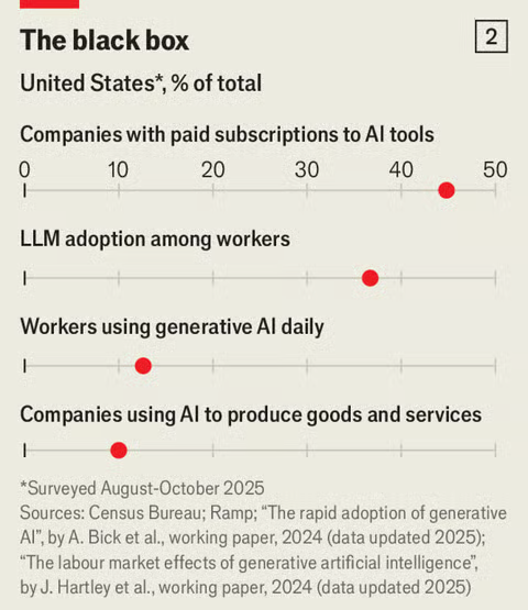
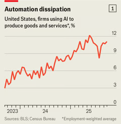
Honored that our paper "The Labor Market Effects of Generative Artificial Intelligence" (with @BrendanDMoore, @FilipJole, & @MeloVitor_) was cited in a new article at @TheEconomist on the 3Q2025 slowdown of Generative AI adoption (article by @econcallum) economist.com/finance-and-ec…
1
6
27
3,671
Capitalism and Freedom in the 21st Century Podcast retweeted
18 Nov 2025
THE TAYLOR RULES:
1. Economic policy should aim to increase economic stability and economic growth.
2. Official finance should support good economic policy with strong ownership. It cannot substitute for bad economic policy.
3. Raising productivity growth is essential for reducing poverty. This requires economic freedom that eliminates impediments to efficient allocation of capital and labor and to the spread of technology.
4. The private sector — not the government — is the engine of economic growth.
5. The international financial system works better when official lending decisions and sovereign debt restructuring processes are predictable. This encourages more efficient movement of capital and a lower cost of capital.
6. Contagion is not automatic. It can be contained by good policy, dissemination of information, and greater predictability in the international financial system.
7. Loans should not be made when there is a high probability that they will be forgiven. Assistance for the poorest countries should be in the form of grants, not loans.
8. Development assistance must produce measurable results. All donors should set clear goals and timelines. Success should be measured by whether these goals and timelines are met, not by the volume of disbursements.
9. Monetary policy should focus on price stability. Sound exchange rate policies support this objective, prevent crises, and allow adjustment throughout the global financial system.
10. Tax systems with broad bases, efficient administration, and low marginal rates are best to encourage both growth and sustainable public finances.

1
16
54
4,370
Capitalism and Freedom in the 21st Century Podcast retweeted
14 Nov 2025
Science!

2
2
34
2,657
Capitalism and Freedom in the 21st Century Podcast retweeted

17 Oct 2025
Based.

9
28
240
86,727
Capitalism and Freedom in the 21st Century Podcast retweeted
13 Oct 2025
NIH Director @DrJBhattacharya joins Hoover Policy Fellow @Jon_Hartley_ on @CapAndFreedom to discuss his vision for the National Institutes of Health, running it as an innovation accelerator, replication in the sciences, the new NIH policy reducing animal testing, and more.
8
9
62
25,057
Capitalism and Freedom in the 21st Century Podcast retweeted
13 Oct 2025
NIH Director @DrJBhattacharya joins the @capandfreedom podcast; we talk his vision for the @NIH & running it as an innovation accelerator. Timely conversation given today's @NobelPrize in Economics for innovation-driven growth. Also the NIH has seriously reduced animal testing!
13 Oct 2025
NIH Director @DrJBhattacharya joins Hoover Policy Fellow @Jon_Hartley_ on @CapAndFreedom to discuss his vision for the National Institutes of Health, running it as an innovation accelerator, replication in the sciences, the new NIH policy reducing animal testing, and more.
2
3
16
4,148
Capitalism and Freedom in the 21st Century Podcast retweeted

2 Oct 2025
This one was hard to write, personally.
I hope you enjoy it.
"Designed for Weakness: The European Commission's leadership problem"
siliconcontinent.com/p/desig…
2
12
50
5,441
Capitalism and Freedom in the 21st Century Podcast retweeted

12 Sep 2025
A couple of days ago, I posted on the double descent phenomenon to alert economists about its importance.
To illustrate it, I used the following example:
1️⃣ You want to find the curve that “best” approximates an unknown function generating 12 observations.
2️⃣ I know the target function is
Y = 2(1 - e^{-|x \sin(x^2)|}), but you do not. You only know there is no noise in the problem.
3️⃣ You use, as an approximator, a single-hidden-layer neural network with ReLU activation trained on these 12 observations.
4️⃣ You check what happens with the approximation when you increase the number of parameters in the neural network from 4 to 24,001.
🎥 The gif movie my dear coauthor @MahdiKahou prepared illustrate the results:
Case A. With a small number of parameters (say, 7), you do poorly: the ℓ₂ distance between your trained approximation (blue line) and the target function (not plotted, only the 12 red points drawn from it) is high.
Case B. With ~1,000 parameters, you reach the interpolation threshold: the network perfectly fits all 12 points, but the function is very wiggly. The ℓ₂ distance is still high.
Case C. With even more parameters (e.g., 24,001), the approximation smooths out, and the ℓ₂ distance to the target function becomes much smaller.
⚡ Key points:
1️⃣ This is just one example, but similar results have been documented in thousands of applications. I am not claiming any novelty whatsoever here.
2️⃣ The result does not hinge on having exactly 12 observations (with more, double descent appears sooner), on noise being absent, or even on using neural networks—you get it with many other parametric approximators.
3️⃣ Yes, in thousands of economic applications, you want to approximate complicated, high-dimensional functions with all types of intricate shapes, and you only know a few points drawn from them.
👉 Why prefer the smooth approximation? Because, even if overparametrized, it generalizes better. If I draw new observations from the (unknown to you) target function
Y = 2(1 - e^{-|x \sin(x^2)|}),
the neural network with 24,001 parameters will forecast them better (on average) than the one with 1,000 parameters.
The original post is here:
x.com/JesusFerna7026/status/…
A (partial) explanation of what is going on is here:
x.com/JesusFerna7026/status/…
For many more details, read the breakthrough paper by Belkin et al. (2019):
pnas.org/doi/10.1073/pnas.19…
and some recent interesting papers:
arxiv.org/abs/2303.14151
arxiv.org/abs/2503.02113
11 Sep 2025

In my post yesterday, I described the double descent phenomenon: in many situations, massively over-parametrized models outperform simpler models out of sample. As I emphasized, this is one of the most surprising and intriguing developments in computer science and statistics in recent decades and it has important implications for economics.
The double descent phenomenon raises many questions, most still unanswered or only partially answered, despite intense work by top researchers. Today I will sketch one key element of the emerging picture: the inductive bias of deep learning. This requires some work, so please stay with me.
When a model is heavily over-parametrized (for example, as I mentioned yesterday, with 12,001 parameters for 12 observations), there are many parameter configurations that interpolate the data, i.e., they fit all 12 observations perfectly.
Which parameters are selected in practice? In high dimensions, gradient-based optimizers that minimize fit loss often converge to minimum-norm (min-norm) interpolants under the relevant function class/parameterization. In linear settings (and several over-parameterized regimes/initializations for neural networks), this can be proved; more broadly, practice shows a strong implicit bias toward min-norm solutions.
What does that mean? Think of the fitted model as a function (the curve that goes exactly through all 12 points). The optimizer effectively selects the curve that is “smoothest” in a well-defined sense: the curve that minimizes a functional seminorm (e.g., a Sobolev seminorm).
What is a functional seminorm? A basic mathematical task is to measure the “size” of an object (like the length of a vector).
A norm is just a concept of “size” that is useful for the task we are dealing with. That is why in high-school math we introduce ideas like the Euclidean norm of a vector: it gives us a very intuitive and useful way to think about the “size” of a vector.
Norms can be too strict for many problems; sometimes we want a size that treats certain nonzero objects as “equivalent to zero.” A seminorm does exactly that: it measures size while allowing some nonzero objects to have size zero.
A functional seminorm applies this idea to functions, giving a way to quantify the size of the whole function, not just its value at a point (though pointwise evaluation can itself be used as a seminorm).
Enter Sobolev seminorms (and their relatives): here, the “aspect” of the function we measure is smoothness—how large its derivatives are. A Sobolev seminorm ignores baseline level and measures only the magnitude of derivatives; it is a seminorm because adding a constant (or, for higher orders, a lower-degree polynomial) does not change it.
A metaphor: imagine rating the difficulty of a bike trail for your weekend excursion. You want to assess the entire trail, not a single point. The Sobolev seminorm “measures” the curvature, wiggles, and twists of the trail, but it does not care whether the trail sits at 100 or 500 meters above sea level.
There are many reasons Sobolev seminorms matter across mathematics. For example, if you’re solving the heat equation for a rod, you care about how steep the temperature gradient is along the rod, not how hot the rod is.
But the key point for us is that they give an intuitive measure of how smooth a curve is.
Now return to the figure from my post yesterday:
x.com/JesusFerna7026/status/…
Of all neural networks with 12,001 parameters that fit the 12 observations perfectly, a gradient-based optimizer tends to pick the smoothest one (in the sense above). That is the inductive bias at work, and it’s remarkable.
The formal statement is in the snapshot from my paper:
x.com/JesusFerna7026/status/…
included in this post.
We can prove this behavior in a number of cases; in practice, it appears beyond those instances as well. This is why yesterday’s example was not cherry-picked.
Why do we care about “smooth” curves?
1️⃣ Occam’s razor. Smooth curves are typically the simplest, delivering an inductive bias toward simplicity.
2️⃣ Dynamic economic models. The smooth solutions are precisely those that satisfy the transversality condition. I have a full paper on this:
sas.upenn.edu/~jesusfv/Spook…
I will explain more another day.
3️⃣ Forecasting. In practice, smoother curves generalize better and forecast new observations more accurately.
Finally, a quick diagnostic from the figure: the ℓ₂ distance between the true function and the interpolated solution is much smaller in panel 4 than in panel 3. That is, the massively over-parametrized solution (panel 4) outperforms the merely overfit solution (panel 3) precisely because the massively over-parametrized solution minimizes the seminorm.
I realize this post likely opens more questions than it answers (and I had to be a bit sloppy with some details), but bear with me—I’ll try to address those next week.

5
39
181
28,761
Episode 59. Cass Sunstein on Nudges, Behavioral Economics, Law, and Liberalism hoover.org/research/cass-sun…
1
1
3
689
Full Transcript: capitalismandfreedom.substac…
66