
Spineless Coding Agent Amateur
Joined April 2026
- Tweets 75
- Following 31
- Followers 14
- Likes 111
10 Photos and videos


ForthMFS retweeted
Is Parallel Programming Hard, And If So, What Can You Do About It?
mirrors.edge.kernel.org/pub/…

25
161
4,866

Built moongrep, an experimental structural code search tool for MoonBit.
Run it with a single `moon runwasm moonbit-community/moongrep@0.1.5` command — no manual compilation needed, and it works cross-platform!
#moonbit #moonbitlang
1
20
ForthMFS retweeted

Jun 14
One of the best free courses on low-level performance programming - Aalto University's Programming Parallel Computers covers SIMD, pipelining, cache optimization, and more.
If you care about squeezing CPU cycles, this is definitely worth taking up.
ppc.cs.aalto.fi

111
822
47,313
ForthMFS retweeted
Jun 9
Interesting...
sigops.org/s/conferences/sos…

Jun 9

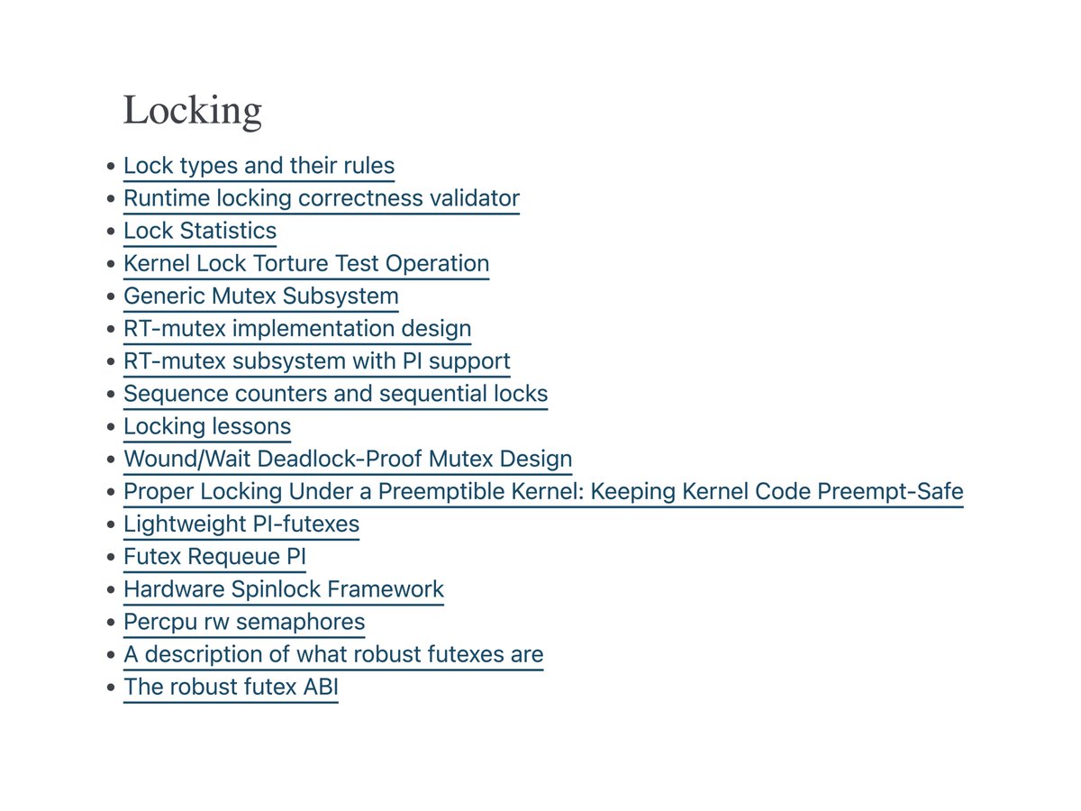
Great docs on Kernel's way of handling concurrency - the bridge between the theory (QT) and the practical implementation!
docs.kernel.org/locking/inde…
31
197
7,339
ForthMFS retweeted

Jun 7
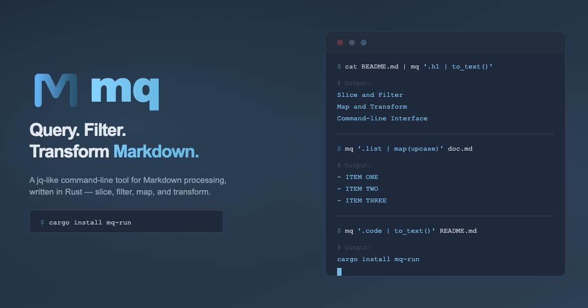
harehare/mq - A jq-like Markdown query language for command-line processing #devopsish github.com/harehare/mq
2
22
198
15,213
ForthMFS retweeted
Jun 6
Andy Grove's "How Query Engines Work" is a great free resource as a hands-on guide to building a query engine from scratch.
howqueryengineswork.com

Jun 6
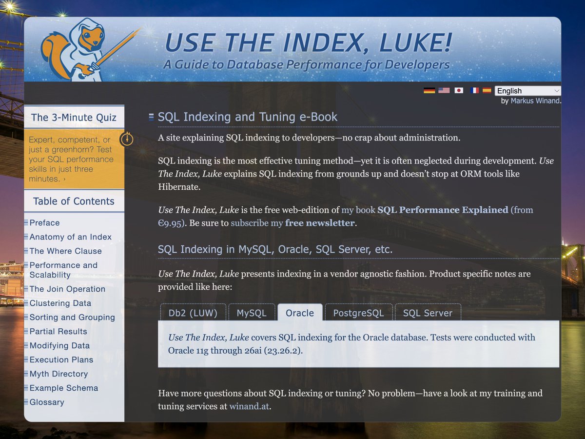
SAVE this - "Use The Index, Luke" is a comprehensive, free educational resource focused on SQL indexing and performance tuning for developers.
use-the-index-luke.com/
1
41
349
15,477
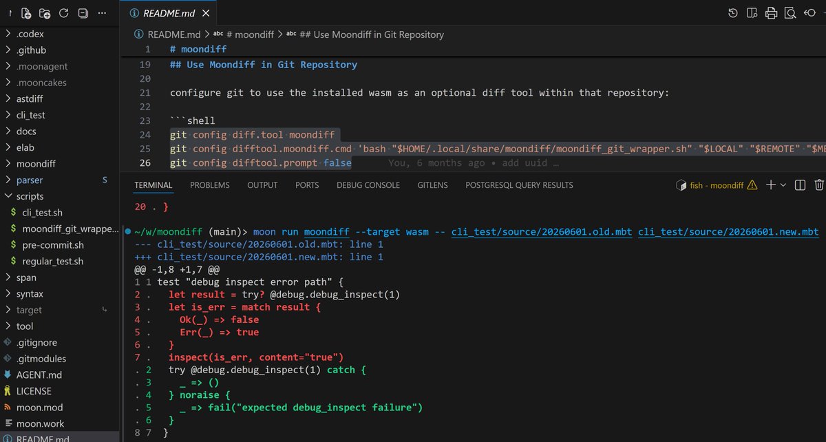
Built an AST diff tool for MoonBit, hope it will eventually become useful: moonbit-community/moondiff
#moonbit #moonbitlang
1
12
1,632
ForthMFS retweeted

Jun 4
In the stable release of @moonbitlang
And the coming releases
We are experimenting v128 support, stay tuned 🚀🚀🚀

4
13
6,745
ForthMFS retweeted

Jun 1
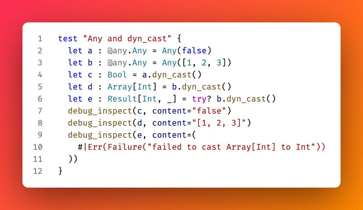
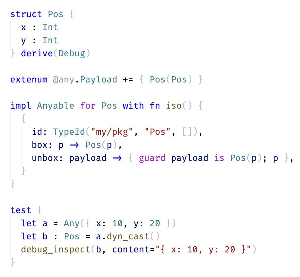
Any downcast isn’t supported in MoonBit yet due to wasm-gc limitations.
Current workarounds use unsafe intrinsics or JSON conversion, but that either gives up Wasm-gc or hurts performance.
Any better workaround? Check this:
mooncakes.io/docs/Yoorkin/an…
1
1
14
1,055
ForthMFS retweeted
May 28
In the stable release of @moonbitlang
We've switched the ABI of `println` to wasip1 when building an executable (`fn main`), hoping that it will increase compatibility so that people no longer need to fear of it.
The escape hatch is `MOON_WASI_LINK=0`.

1
3
13
5,001
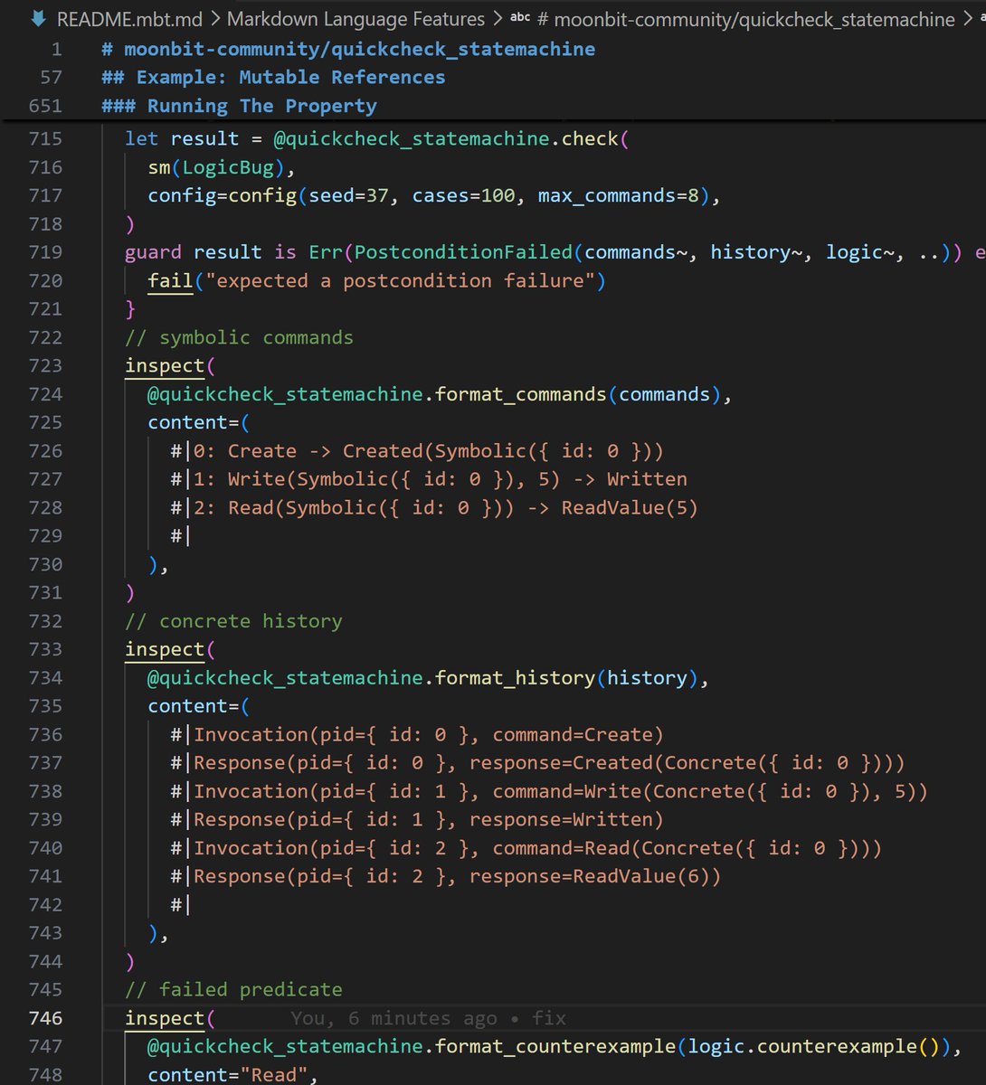
Use github.com/moonbit-community… to write property-based tests for stateful MoonBit programs.
#moonbit #moonbitlang
3
909
ForthMFS retweeted

May 28
Please check moonbitlang.com
I once spent a long time building the language I wanted for myself, and it happened to hit exactly the properties you mentioned, along with a type system expressive enough. when I knew MoonBit, I realized it was what I wanted
- fast like C
- memory safe like Rust
- fast compilation like Go
- 1st class C support like Swift
Who’s building this?
2
6
219
ForthMFS retweeted
May 27
Beginner's Guide to Linkers - the definitive reference for understanding what's actually happening when you link.
lurklurk.org/linkers/linkers…


2
92
651
42,196

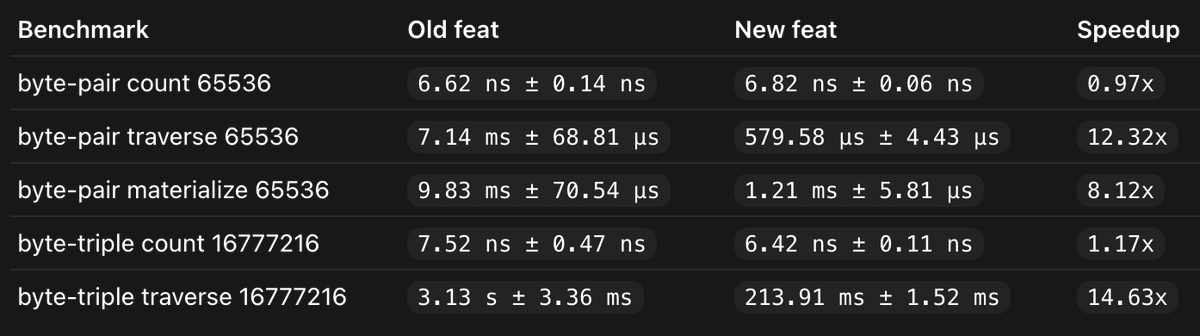
Replacing MoonBit QuickCheck FEAT with a new implementation significantly improves its performance.
The key is using IFSeq to represent finite parts, preserving random access, providing direct foreach paths for traverse/materialize, and a prefix cache to the global index.
2
8
1,112

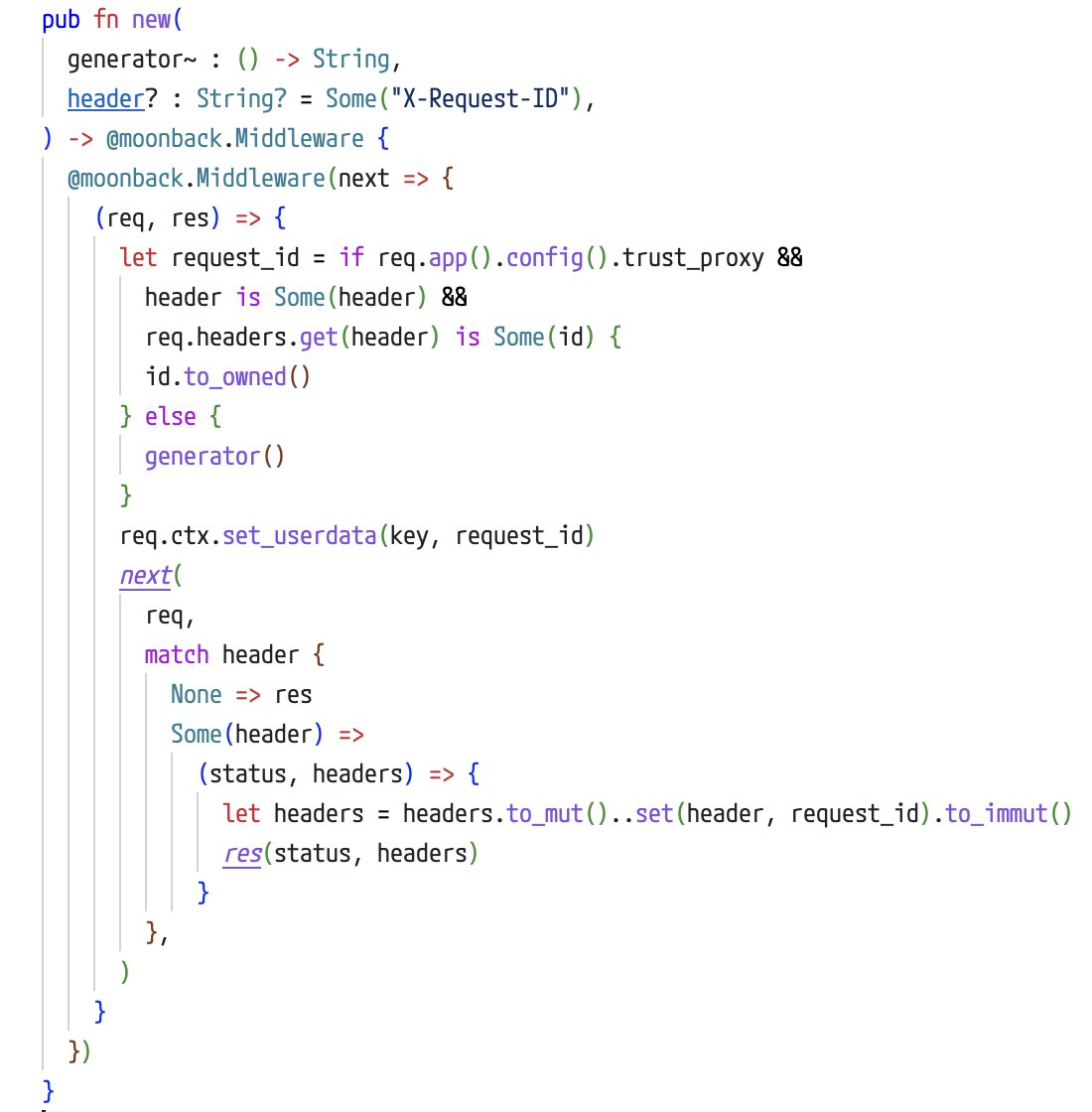
This is the request_id middleware in #moonback.
I like the new copy-on-write Headers/MutHeaders design. It's simple and elegant.
@moonbitlang
2
7
1,169
ForthMFS retweeted
May 26
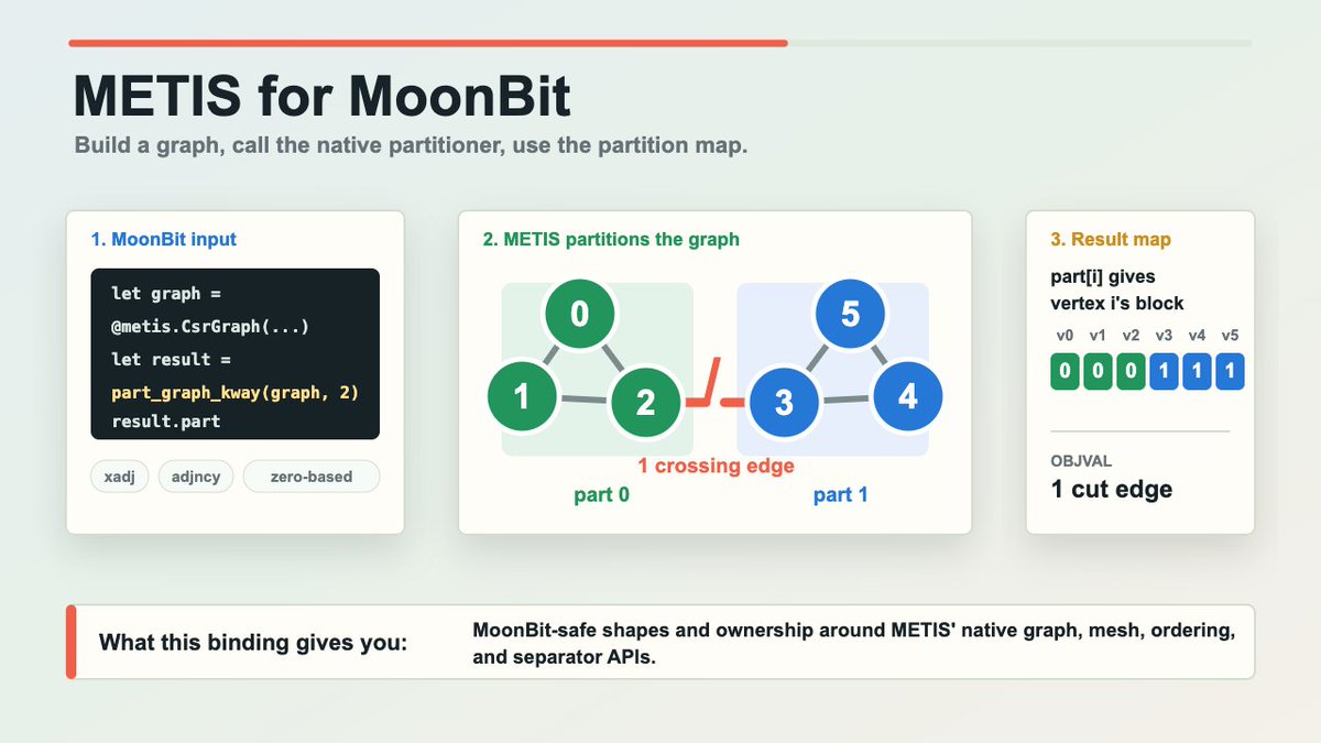
Use Milky2018/metis in your MoonBit projects for graph partitioning, finite-element mesh partitioning, and fill-reducing ordering.
It is especially useful for scientific computing, sparse matrix preprocessing, and scheduling parallel workloads.
#moonbitlang
2
6
3,911
ForthMFS retweeted

May 26
"Because we don't necessarily know at this point"
- commit from 2004 that still exists in Postgres today.
The below screenshot is from the `analyze.c` file in the Postgres source code. The number 300 is a hardcoded value inside of Postgres's ANALYZE code. The rationale is based on a paper entitled "Random sampling for histogram construction: how much is enough?" written in 1998 when data sizes were much smaller and hardware was much slower. The question the paper answers is: to build statistics enabling optimization of queries of unindexed data, how many rows does ANALYZE need to sample to build accurate enough statistics?
The answer is 300-ish samples for each bin you want in your equi-height histogram. Why? The paper shows that required sample size grows linearly with the number of bins but only logarithmically with table size for most cases, so you see diminishing returns beyond a few hundred samples per bin.
For instance, the default `statistics_target` is 100. That means Postgres aims to sample 300 x 100 values to build an equi-height histogram with 100 bins and while also storing the 100 most common values.
(Check out the previous post for deets on how Postgres uses equi-height histogram and most common values)
Why all this work for unindexed data?
Because in 1998, indexes were extraordinarily costly to build and maintain. Indexes took up valuable disk space, used the limited IOPs during writes and builds. Additionally table scans were slow and blocking. In 1998, hard drive performance was measured in RPMs, so talking IOPs was variable because random page seeks required waiting for the disk to rotate, and location on disk was unknown. The tests for this paper ran on Pentium 200MHz with 64MB of RAM, and a 7.2k RPM SCSI drive.
Postgres users continue to benefit from this work during the era of constrained resources. Indexes aren't free today, and you can have too many indexes, but they aren't as costly as they were. Also, unindexed data isn't as costly as it was.
The paper also acknowledges the problem is "provably difficult by establishing a limit on the achievable accuracy of estimation in the worst-case." Thus, "we devise a simple estimator which we believe is optimal." This number is a tradeoff between accuracy and performance. A smaller multiplier would lead to less accurate statistics, which could cause the planner to make bad decisions. A larger multiplier would lead to more accurate statistics, but it would also make ANALYZE slower. And remember, ANALYZE was much, much slower back then.
What does statistics_target control?
The statistics target controls the number of values stored for Most Common Values and the Equi-height Histogram. The following is true:
```
statistics_target = 100 → 30,000 samples, 100 MCVs, 100 buckets
statistics_target = 500 → 150,000 samples, 500 MCVs, 500 buckets
statistics_target = 1000 → 300,000 samples, 1000 MCVs, 1000 buckets
```
This value is set by default at the database level, and can be overridden at the column level.
```
-- Per-column override:
ALTER TABLE requests ALTER COLUMN status_code SET STATISTICS 500;
ANALYZE requests;
```
For larger databases, there is usually at least one column where a per column setting may be the right approach. Don't raise the global default just because one column needs more granularity. Given the performance gains of the underlying hardware, the performance gains from changing column statistics aren't as significant as they once were.

2
17
184
25,784
ForthMFS retweeted

May 24
Has been a while since I wrote about agentic engineering, so this time around some learnings of maintaining Pi as a junior maintainer to @badlogicgames :) lucumr.pocoo.org/2026/5/24/p…
29
81
908
147,903
ForthMFS retweeted

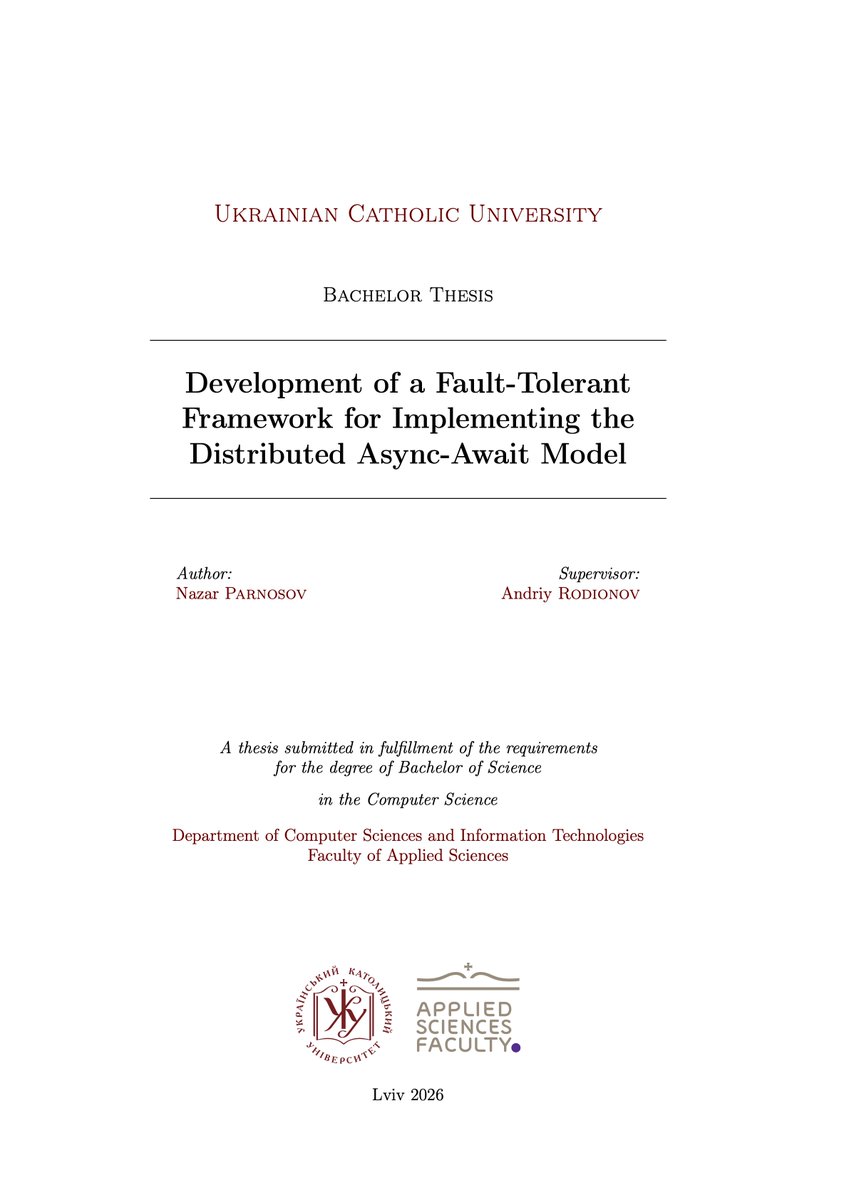
May 25
Resonate entered academia: Nazar Parnosov wrote his bachelor thesis on Distributed Asynchronous Await
Imagine my surprise when he dropped his thesis in the @resonatehqio Discord ❤️
2
9
105
5,895
ForthMFS retweeted
May 25
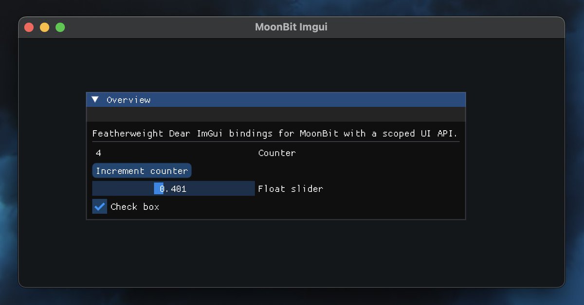
Experimenting with a scoped UI wrapper for MoonBit Dear ImGui bindings. It’s like a trailing-lambda UI API, but more featherweight
github.com/moonbit-community…
#moonbit #imgui

3
11
4,802