
AI/ML. Worked at Meta, Uber, Amazon, Apple, and Microsoft building apps, developer platforms, and hardware. Tweeting about LLM psychotherapy.
Joined August 2008
- Tweets 21,398
- Following 397
- Followers 5,844
- Likes 521
2,558 Photos and videos


Pinned Tweet

26 Aug 2025
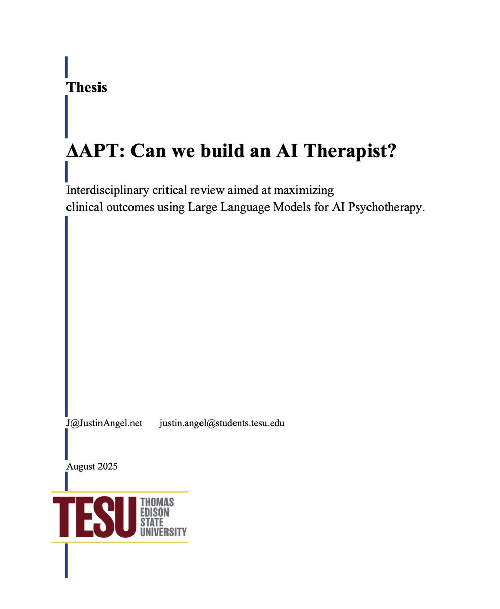
🚨 New Preprint: ΔAPT - Can we build an AI Therapist?
osf.io/preprints/psyarxiv/4t…
LLMs are already powering AI psychotherapy tools (APTs), but are they clinically effective?
This interdisciplinary review frameworks maps architecture design choices to clinical outcomes.
🧵
8
4
321
115,590
Jun 13
This is the first time that while coding I get a popup saying export controls have been activated on a programming tool.
I've been writing code for 25 years.
1
161
Jun 10
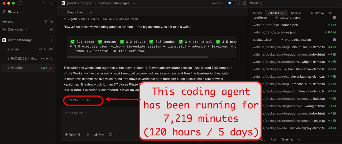
5 days. This coding agent has been running for 5 days.
Writing good specs has always been part of the job of software engineers, it's just the audience that shifted.
(shown here: @conductor_build using claude code Opus 4.8 max running parallel agents and subagents).
116
Jun 3
GPUs go brrrrrr when they dream of us

1
142
Jun 2
During NEO @swyx casually dropped "you can make custom ribbons for @aiDotEngineer in SF".
Challenge accepted.
2
10
11,506
May 23
Live streaming the recording of the Build your own LLM workshop @ x.com/i/broadcasts/1pKkOOymZ…
(with breaks during the day)
1
1
14,639
May 21
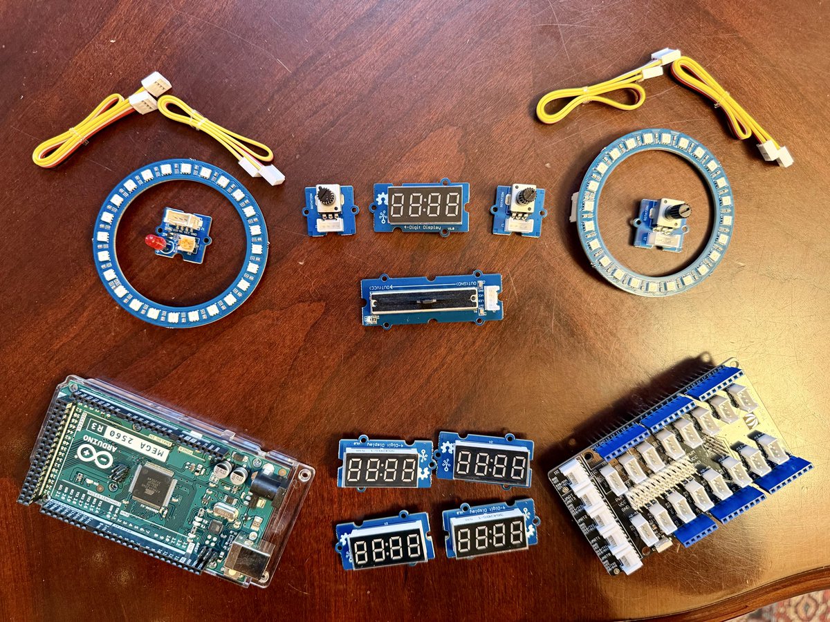
I've solidified a neural net perceptron into a physical circuit. 100 billion of these is ChatGPT.
f(x)= wx b = 1*1 1.5 = 2.5
output = weight * input bias
You can change the input, weight and bias and see the output neuron update.
Learning ML can be fun!
5
5
38
97,933
May 21
Also added a ReLU max(0,x) function to more closely resemble GPT-2.
f(x) = w*x b = -1.5 * 2 2 = -1
When numbers go negative, the final output is still 0.
So max(-1, 0) -> the final output is 0.
1
247
May 21
Play around with the circuit yourself @ go.justinangel.ai/neuralnet
Used in my "Build your own LLM" course to teach about perceptron, neural nets, and back-propogation.
Heavily inspired by @welchlabs and @ProfTomYeh.
1
184
Justin Angel retweeted

May 18
Most unsupervised "feature discovery" in LLMs uses sparse auto-encoders, which work, and which have been scaled to millions of features on frontier-scale models, but which bundle two distinct commitments – a reconstruction loss and a sparsity loss over a fixed-size dictionary – into a single training objective.
Those commitments make sense if your goal is reconstructive decomposition. They make less obvious sense if your aim is to find interpretable structure (directions? features?) in activation space, to retrieve representative examples, identify causal interventions, or measure how representations change across layers and inputs. It turns out a lot of that doesn't need the full SAE machinery.
Exemplar Partitioning (EP) uses leader-clustering (Hartigan, 1975!) to cover the activation manifold with observed exemplars at a calibrated resolution, resulting in a Voronoi partition of activation space that you can read like a feature dictionary.
EP makes one streaming pass over the data until saturation (when no new exemplars form), and uses no backward passes or gradient descent. The animation above shows the algorithm – each new activation either joins an existing cell (close enough to an exemplar) or seeds a new one. It's extraordinarily simple and cheap.
On AxBench latent concept detection at Gemma-2-2B-it L20, EP reaches 0.881 mean AUROC across 500 concepts. That's within 0.03 of SAE-A (AxBench's strongest dictionary-based baseline), and 0.126 over the canonical GemmaScope 16k SAE leaderboard entry – with about 1,000× less build compute.
And you can do a lot interesting stuff with the resulting dictionary!
If you build it on a mix of harmful and benign prompts, one region absorbs most of the refusing prompts. Projecting held-out harmful prompts off that exemplar's direction collapses refusal from around 0.98 to around 0.02 – the same ballpark as dedicated refusal-direction work (Arditi et al., 2024).
If you build the EP dictionary to saturation on a corpus (e.g. the Pile), distance-to-nearest-exemplar becomes a graded measure of distribution shift, for free. Random-token-sequence activations sit measurably further out than Pile activations, and Bulgarian Wikipedia (under-represented in the Pile but not really OOD) sits between the two.
Because exemplars are real activations rather than learned decoder columns, you can match dictionaries across different models by their exemplars. If you match EP dictionaries from base vs instruction-tuned Gemma-2-2B, only a handful of regions survive as common, mostly general-purpose syntactic patterns. You can also see how the base model already represents "harmful" as a direction at earlier prompt positions, and instruction tuning pulls it forward to the final-token activation where the refusal decision is made.
The saturated size of a dictionary on a given input stream is itself a measurement of that stream's activation geometry at each layer. On the same model, the proportion of activation space dedicated to chat grows monotonically with depth, code is essentially flat across the network (and lives in a smaller area of activation space than chat does, at every layer), and math is non-monotonic, peaking in the middle.
EP and SAEs don't converge on the same features, aside from a shared core of about 20%. The two methods make different geometric commitments – SAEs to linear separability, EP to density.
The experiments I've done so far are small-scale and exploratory, and I have only tested on Gemma-2-2b. There's a huge amount of further work to be done (both in terms of improving the method and applying it to more tasks), some of which is discussed in the post and paper.
If you are an interpretability researcher interested in developing this method please check out the github repo and get stuck in!
Post: lesswrong.com/posts/RroeHBSk…
Paper: arxiv.org/abs/2605.14347
Code: github.com/jessicarumbelow/e…
3
4
69
3,530
May 17
Light weekend reading focus on overviews of pragmatic mechanistic Interpretability. As opposed to the inactionable and impractical kind I guess?
Locate, Steer, and Improve: A Practical Survey of Actionable Mechanistic Interpretability @ arxiv.org/abs/2601.14004
Practical Review of Mechanistic Interpretability @ arxiv.org/abs/2407.02646
1
2
223
Justin Angel retweeted
May 16
Voronoi partitions on activations reveal interpretable structure with orders of magnitude less compute than SAEs! Here is an introduction to a new interpretability method: lesswrong.com/posts/RroeHBSk…
5
29
261
25,920
Justin Angel retweeted
May 14
My guess is that this policy will be applied selectively depending on institutional privilege and personal notoriety. It'll end up as a tool of silencing unconnected individuals vs. promoting better scientific discourse.
I aspire to be wrong.
19
3
195
35,396

I took a Build Your Own LLM workshop. Here's my review: emilyhk.com/llm-workshop/ @JustinAngel @leecflannery
1
1
182
May 11
Prompt Gemini: “Continue (1000 characters): ATCGAAA” goes on forever.
LLM functions are wild.
The problem with having your LLM loss function as next token prediction is that some things don’t have natural ends in training data. Like, DNA notation.
GPUs go brrrrrrrr
1
258