
Scientific strategist | Storyteller | Genomics, Lab diagnostic and high throughput automation | Coder | Comments are my own
Joined October 2008
- Tweets 38,426
- Following 3,964
- Followers 9,970
- Likes 22
19 Photos and videos


16 Aug 2023
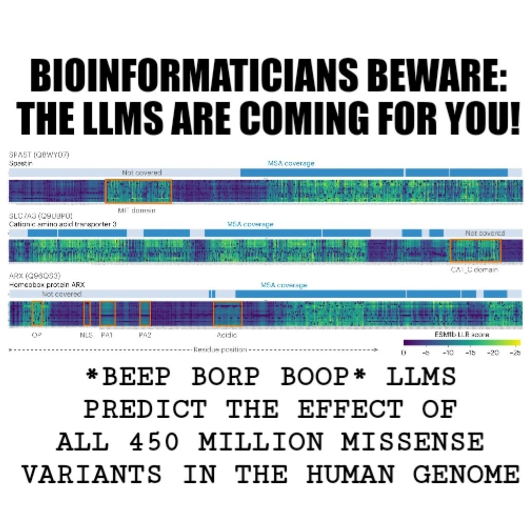
Can LLMs predict the effects of all potential missense variants in the human genome?
Predicting the effects of genetic variants on human proteins can be quite challenging.
Existing methods struggle to accurately distinguish between harmful and benign variants, especially when it comes to missense variants that substitute one amino acid for another.
Here, the authors explored two approaches: experimental methods like deep mutational scans (DMS), and computational methods like unsupervised homology-based techniques and protein language models (PLM).
While DMS can capture molecular and cellular phenotypes, they have scalability challenges and are imperfect proxies for clinical outcomes.
Alternatively, computational methods leverage protein properties and evolutionary constraints, but most are trained on labeled data, limiting their coverage.
One such computational approach is EVE, an unsupervised deep-learning method based on generative variational autoencoders, but its predictions are constrained to well-aligned proteins.
This study focused on ESM1b, a neural network based protein language model trained on millions of protein sequences. ESM1b's advantage lies in its ability to predict variant effects without relying on explicit homology, covering a broader range of variants.
The researchers developed a workflow to use ESM1b to predict the effects of all possible missense variants in known human proteins. They evaluated their approach on various benchmarks and compared it with other variant effect prediction methods.
The results showed that ESM1b outperformed other methods in classifying variant pathogenicity.
The most impressive of these was ESM1b's ability to predict variant effects across different protein isoforms. The authors state that it was able to, “distinguish between pathogenic and benign variants [and] yield a true-positive rate of 81% and a true-negative rate of 82%.”
However, ESM1b struggled with variants that led to nonsense-mediated decay (NMD), and the study utilized a sliding window approach for lengthy proteins, which could miss distant interactions. Validation against more experimental data will be crucial before applying ESM1b in real-world scenarios.
The emergence of LPLMs like ESM1b offers a promising avenue for predicting variant effects. These models could improve diagnostic accuracy, aid genetic association studies, inform protein engineering, and uncover new insights into protein function.
As LPLMs continue to advance, they hold promise for enhancing our understanding of genetic variants and their impacts on human health.
###
Brandes N, Goldman G, Wang CH et al. 2023. Genome-wide prediction of disease variant effects with a deep protein language model. Nat Genet. DOI: 10.1038/s41588-023-01465-0
🤖 This post was mostly written by ChatGPT. It only seemed right to let the LLM write about LPLMs. 🤖
I fixed all of the weird things it got wrong - like the most important result in the paper. 😬
2
1
4
657
11 Aug 2023
Nettie Stevens discovered sex chromosomes in 1905. This former school teacher became a genetics pioneer that you need to know!
The late 1800s were a turning point in American history for women. The end of the Civil War marked the start of the women's rights movement and granted them significantly more control over their own lives.
That being said, women were still expected to be teachers or home makers but they won more personal freedom including better access to education.
Nettie Stevens took advantage of these expanded liberties, and started her educational pursuits at age 10 studying to become a school teacher.
In 1883, she began a decade-long career in education, filling roles both as a teacher and as a librarian.
However, this wasn't her life's dream, and in 1896, at the age of 34, she had saved enough money to enroll at Stanford University earning both her bachelor's and master's degrees in 1900.
It was during her summer studies that she took a keen interest in cytology while working at the Stanford Marine Lab. Here she spent her time glued to a microscope and published her first paper on the life-cycle of ciliates in 1901.
Stevens then left Stanford to continue her scientific studies at Bryn Mawr beginning her dissertation work under the guidance of Thomas Hunt Morgan.
You might be familiar with him.
Morgan received the Nobel Prize in 1933 for his work elucidating the role of chromosomes in heredity.
Interestingly, Morgan was initially skeptical of heredity, particularly as it related to sex determination.
At the time, there were two competing hypotheses. One being that sex was determined by environmental factors, like temperature, and another that sex was inherited as a trait.
In spite of the lingering questions on this topic, Stevens successfully completed her dissertation in 1903, and received an award from the Carnegie Institution to study how sex is determined.
This work is the subject of today's #FigureFriday wherein Stevens meticulously detailed the cellular structures of the reproductive organs of multiple insects.
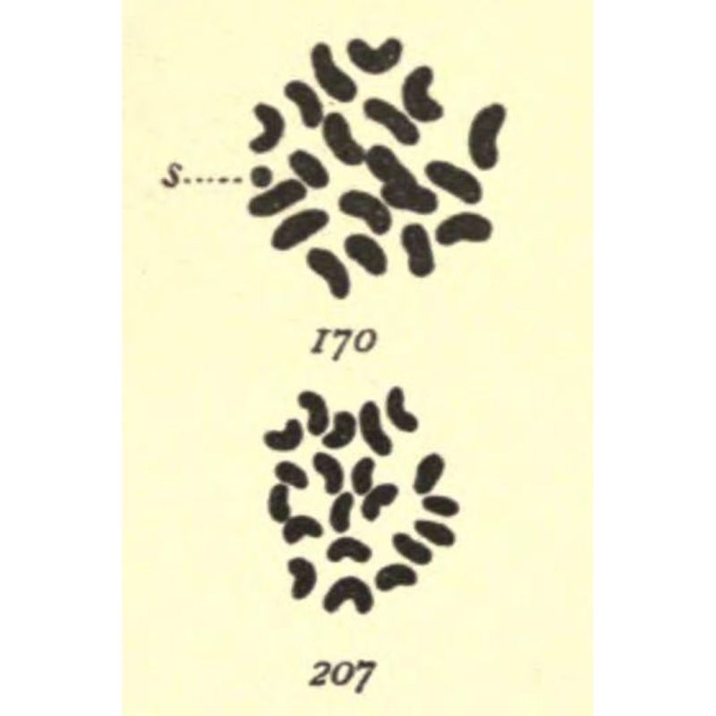
The most striking of these being her drawings in 1905 of the chromosomes found in mealworms (Tenebrio molitor) where she observed:
‘In both somatic and germ cells of the two sexes there is a difference not in the number of chromatin elements, but in the size of one, which is very small in the male (170-s) and of the same size as the other 19 in the female (207).’
Even though she was the first to make this discovery, Thomas Hunt Morgan and another contemporary, Edmund Beecher Wilson, are often incorrectly given the credit.
Tragically, breast cancer cut her life and scientific career short at the age of 50.
But Nettie Stevens' contributions to our understanding of sex determination, along with her exquisite drawings, were the definition of groundbreaking in the field of genetics.
###
Stevens NM. 1905. Studies in Spermatogenesis with Especial Reference to the Accessory Chromosome. Carnegie Institution.
1
1
5
2,325
11 Aug 2023
Here's a link to the paper if you're interested in reading and looking at her really cool drawings: archive.org/details/studiesi…
220
10 Aug 2023
Ethnic stratification and why single reference based analysis methods aren't 'good enough' in 2023.
If you've done genetics for any amount of time you know that stratification of populations is important for getting useful information out of them.
But if you're not a geneticist, it might be a good idea to explain why this is true.
Stratification is a statistical term that basically means "divide your data into subgroups."
In genetics, we usually start with age, gender, life style/exposure, and ethnicity.
The reason for doing this is to be able to determine if subpopulations within a dataset are more or less likely to have whatever it is that you're looking for.
This is usually a measurable trait.
Sometimes this is a common trait like height or eye color, but in healthcare, we're usually talking about disease traits.
So, figuring out if a specific gender, age group, or ethnicity is predisposed to a disease is important, but because diverse populations have mostly been absent from clinical studies, it’s hard to identify important markers of disease in them.
While we know ‘variants’ or ‘mutations’ can contribute to disease, how these contribute to disease can differ vastly depending on someone’s ethnic background.
Variants in one ethnicity may not matter in another ethnicity because mutations elsewhere can compensate in some way for those changes.
So, how you go about determining what is or is not a variant can have a serious impact on the conclusions you draw from a dataset.
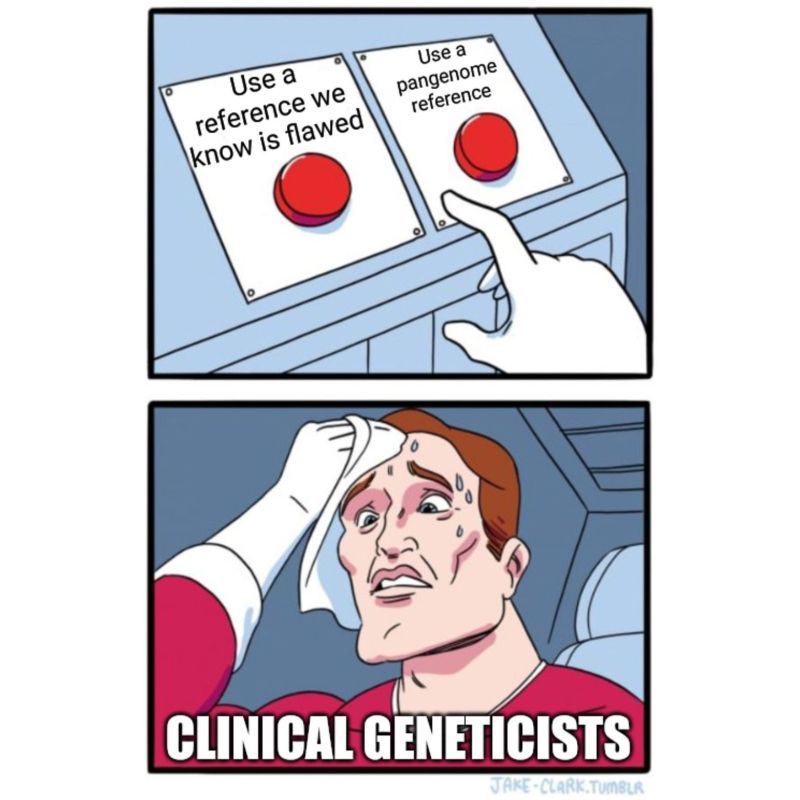
As it stands now, most variants are determined by comparing a patient’s genetic sequence to a ‘reference.’
The reference here is the one determined by the human genome project.
This was supposed to represent the sequence of the average healthy human, but we know now that the bulk of this DNA was provided by a mixed race male.
So ‘variations’ from this reference might not be super accurate if we’re trying to determine the importance of a variant in a different ethnicity.
This bears out in multiple clinical evaluations with a recent survey determining that the number of variants of unknown significance (VUS) was markedly higher in Africans (45%) than Caucasians (32%).
A good chunk of the VUS-ness here has to do with whether the ‘reference’ was appropriate for an African vs a Caucasian, but it also has a lot to do with the fact that most genetic studies have been done in Caucasians, so we already have an idea which ‘variants’ are significant in that population.
Fortunately, we’re seeing progress on multiple fronts here with most associations and government institutions calling for greater diversity in clinical trials.
We also have a human pangenome reference now which more accurately characterizes the ethnic differences we see in our genomes. It’s not completely done yet, but pangenome based variant calling pipelines are available.
So the question is: how long will it take to integrate these updates into clinical practice?
1
2
5
830
4 Aug 2023
While everyone else was distracted by the structure of DNA, Barbara McClintock was figuring out how chromosomes exchange information, and discovered a little thing called the transposable element.
The 1950's were a turning point in the fields of molecular biology and genetics. For many years, scientists studied genetics but weren't entirely sure how it all worked on the molecular level.
They were aware of chromosomes, knew that they were composed of DNA and protein, but there was still a big question about the functional role of those two components in inheritance.
Fortunately for McClintock and other scientists who studied genetics in model organisms - in her case, maize (corn) - it didn't matter much what the genetic material was but that it could be tracked and its effects seen in the offspring of her crosses.
As an early cytogeneticist (a scientist that studies chromosomes), McClintock developed many of the foundational staining techniques that were required for studying chromosomes in maize and she produced the first genetic maps of all 10 chromosomes.
Her early work was focused on studying inheritance and she was one of the first to observe and describe the phenomenon of homologous recombination, or crossing-over, which is when two chromosomes exchange genetic information. She published this work in 1931 and continued to study maize genetics until her curious observation that pieces of chromosome 9 appeared to move around the genome. But these pieces, Ac (activator) and Ds (inhibits pigment production), didn't just move around, Ac seemed to control Ds, and ultimately the color patterns of the maize kernels!
Today's #FigureFriday is an image of the kernels that McClintock described in, 'The origin and behavior of mutable loci in maize.' Kernel 10 - no Ac, 11-13 - 1 copy of Ac, 14 - 2 copies, 15 - 3 copies.
We know today that 66% of the human genome and 85% of the maize genome is made up of these mobile 'transposable' elements and they are key in our understanding of epigenetics, but back in 1950, this discovery was problematic.
At the time, it was thought that genomes were static and ordered; pieces of them did not move around. McClintock's findings were so poorly received that she stopped formally publishing her results after 1953 because she thought her colleagues just weren't interested.
Fortunately, her work was 'rediscovered,' or maybe more accurately, 'understood,' in the 1970's when similar elements were found in bacteria, flies and humans.
She was awarded the Nobel Prize in 1983 for the discovery of transposable elements, which was 3 decades after her original description of them.
McClintock's story in science isn't dissimilar from that of other prominent women, like Rosalind Franklin; however, McClintock lived long enough to finally be properly recognized for her historic achievements.
###
McClintock, B. 1950. The origin and behavior of mutable loci in maize. PNAS: 36 (6) 344-355. DOI: 10.1073/pnas.36.6.344
5
8
1,368
3 Aug 2023
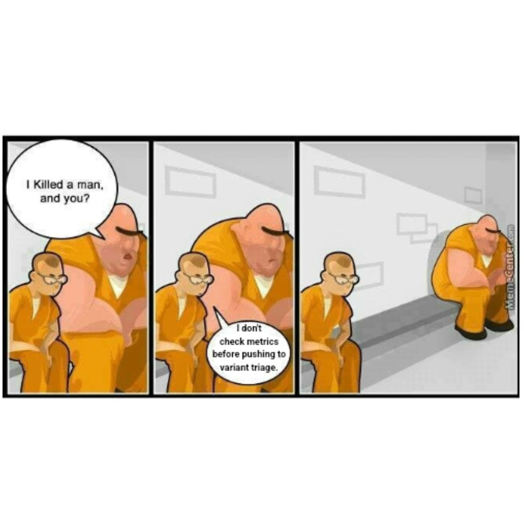
High throughput sequencing metrics: Don't be a monster, review them before sending data to the triage team.
One of the most important things to avoid when doing high throughput sequencing is 'bias.'
Properly assessing your post-alignment and variant calling metrics is super important for ensuring that biased data is not used to generate a patient report.
Here are some of my favorite metrics to keep an eye on:
Percent High Quality (HQ) Reads Aligned - The percentage of HQ reads that actually align to the reference genome. Here HQ is defined as Q20 or better and this stat should be greater than 98%.
GC Bias Plot - This is one of my favorites and for short-read data it should look like an upside down U with high AT and high GC regions showing slight bias (because of amplification) and for long-read methods this plot is usually flat. Any major deviations can indicate bias either from over amplification or if this is target capture data, bias in the capture process.
Insert size - These plots show the size distribution of the sequenced inserts within your library. These should pretty closely mimic the distribution you see in fragment analysis.
Percent Duplication - This is a measure of the number of perfectly duplicated reads in a dataset. The ideal here is less than 5% and usually if you see problems with read duplication you'll also see issues in the GCbias plot.
Coverage - A measure of the average depth of coverage across the genome or your provided target capture probe set.
Transition/Transversion Ratio (TiTv) - Transitions are A<>G or C<>T (substitutions within the purines and pyrimidines) and Transversions A<>C, A<>T, C<>G, and G<>T (conversion of a purine to a pyrimidine, etc). For genomes the expected TiTv is 2 and for exon capture panels it's 3. Major deviations from these values could indicate a bias during sequencing or sample degradation during storage.
Strand Bias - A measure of the bias of the genotype calls made on the positive and negative strands. No bias means calls are the same on each of the complementary strands, high bias means the calls differ and high strand bias around variant calls could indicate an over-reporting of false positives.
Target capture specific metrics:
Fold80 Penalty - This is a measure of evenness or uniformity. The best captures are ones that have perfect uniformity. Fold80 penalty is defined as "fold over-coverage necessary to raise 80% of bases in targets to the mean coverage level." 1 is perfect, so any deviation from that indicates a bias in capture. The best captures are <1.5.
Percent Reads On Target - This is a measure of how much sequencing is being wasted on non-specific binding or off target. This value can vary greatly depending on the size of your capture from 60-70% for an exome down to <20% for smaller capture panels. Deviations from the expected value can indicate bias.
4
3
935
1 Aug 2023
Hey Oncology Market: The proteome is coming at you faster than you think.
One of the early promises that was made during the pitch for funding the human genome project was that once we had figured out the code of life, we'd be able to understand and cure all diseases.
In retrospect, (and even at the time) scientists knew this was hyperbole and that the genome was really just the bottom of the molecular biology pyramid.
Knowing the sequence of the bases is important, but it tells you very little about what is actually expressed by the genome.
For that you need other tools to look at the products of the genome like mRNA, proteins, and metabolites from cellular processes but also modifications to the genome itself that control which parts of it are accessible.
Together we refer to the genome plus all of these other things as the 'multi-ome.'
One of the hardest of these other 'omes' to measure is the proteome.
It represents all of the proteins that make up the little machines that allow our cells to function.
Each of our cells expresses different proteins, and these work together, ultimately creating all of the tissues that make up our bodies.
However, in diseases like cancer, these cellular functions are disrupted due to mutations in the genome that change what is expressed or alter how those proteins function.
We can pick up some of these signals by looking at the genome, but we can get an actual read out of the biology of these cells by looking at the composition of the other 'omes' in the bloodstream!
Up until about 10 years ago, looking at proteins was a very tedious task requiring gels and antibodies or highly complex purification schemes paired with tandem mass spectrometry.
Now we have new techniques for quantifying thousands of proteins at once which gives us a much more comprehensive look at the underlying biology of cancers.
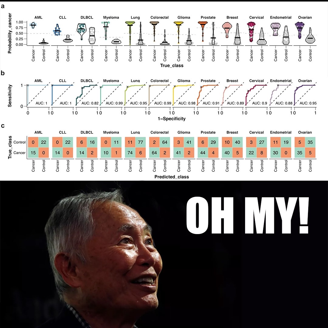
The paper I'm showing a figure from today was written by the group behind the Human Disease Blood Atlas and they characterized 1,463 proteins in more than 1,400 cancer patients.
They then took the data from those results and used machine learning to develop algorithms for predicting AML, ALL, DLCBL, Myeloma, Lung, Colorectal, Glioma, Prostate, Breast, Cervical, Endometrial, and Ovarian cancer.
They followed up by detecting those cancers with relatively high sensitivity and specificity including AUCs for 6 out of 12 above 0.95 (and above 0.8 for the rest!).
While not perfect, this is pretty freakin' good for a first crack, and this work highlights the future potential for proteomics in multi-cancer early detection (MCED).
With some optimization and a more comprehensive method validation, proteomic approaches could make the current players in the MCED space sweat!
###
Álvez MB et al. 2023. Next generation pan-cancer blood proteome profiling using proximity extension assay. Nat Commun. DOI: 10.1038/s41467-023-39765-y
3
7
985
28 Jul 2023
Mendel first described his laws of genetic inheritance in 1865. They were promptly ignored for 35 years.
Because, let's be honest, who gives a husk about peas?!?!
It probably also didn't help that his paper was titled, 'Versuche über Pflanzenhybriden.'
Which in English translates to, 'Experiments in plant hybridization.'
While this sounds exhilarating, it belies the foundational concepts described in its pages and Mendel's work breeding peas wasn't revisited until 1900 when his results were independently rediscovered and confirmed by E. Tschermak (peas), W. Spillman (wheat) and C. Correns (peas).
H. de Vries (flowers) also independently characterized plant genetics in 1900 but had to be told that Mendel scooped him 35 years earlier.
Oof.
So, what was it that Mendel discovered while studying peas?
He observed the physical traits of peas and how these traits were passed to their offspring after breeding.
Mendel established 3 genetic principles from these observations:
Segregation - Traits come in two forms but only one from each parent is passed to offspring.
Independent Assortment - The segregation of the forms of each trait occurs independently of any other trait.
Dominance - Dominant forms of each trait mask the recessive forms and they occur in a 3:1 ratio.
Mendel initially described these as laws, but we know now that there are numerous exceptions, so in genetics we often refer to Mendelian and non-Mendelian inheritance.
But in the early 1900's, the race was on to see if Mendel's phenomenon wasn't just some weird plant thing.
One of the biggest proponents of Mendel at the time was William Bateson.
Bateson is a forgotten figure nowadays, but he popularized the works of Mendel and also did some of the earliest work on genetic linkage.
He also became fast friends with a clinician scientist, Archibald Garrod.
Garrod was most interested in the biology of the diseases in his patients and had a particular fondness for chemistry.
This could be why he was so enamored with the color of his patients’ urine.
This curiosity paid off in 1899 when he first noticed a chemical aberration in the urine of patients with Alkaptonuria.
This is an ancient disease with symptoms being described as far back as 1500 BC, but one of its tell-tale signs is darkly pigmented pee.
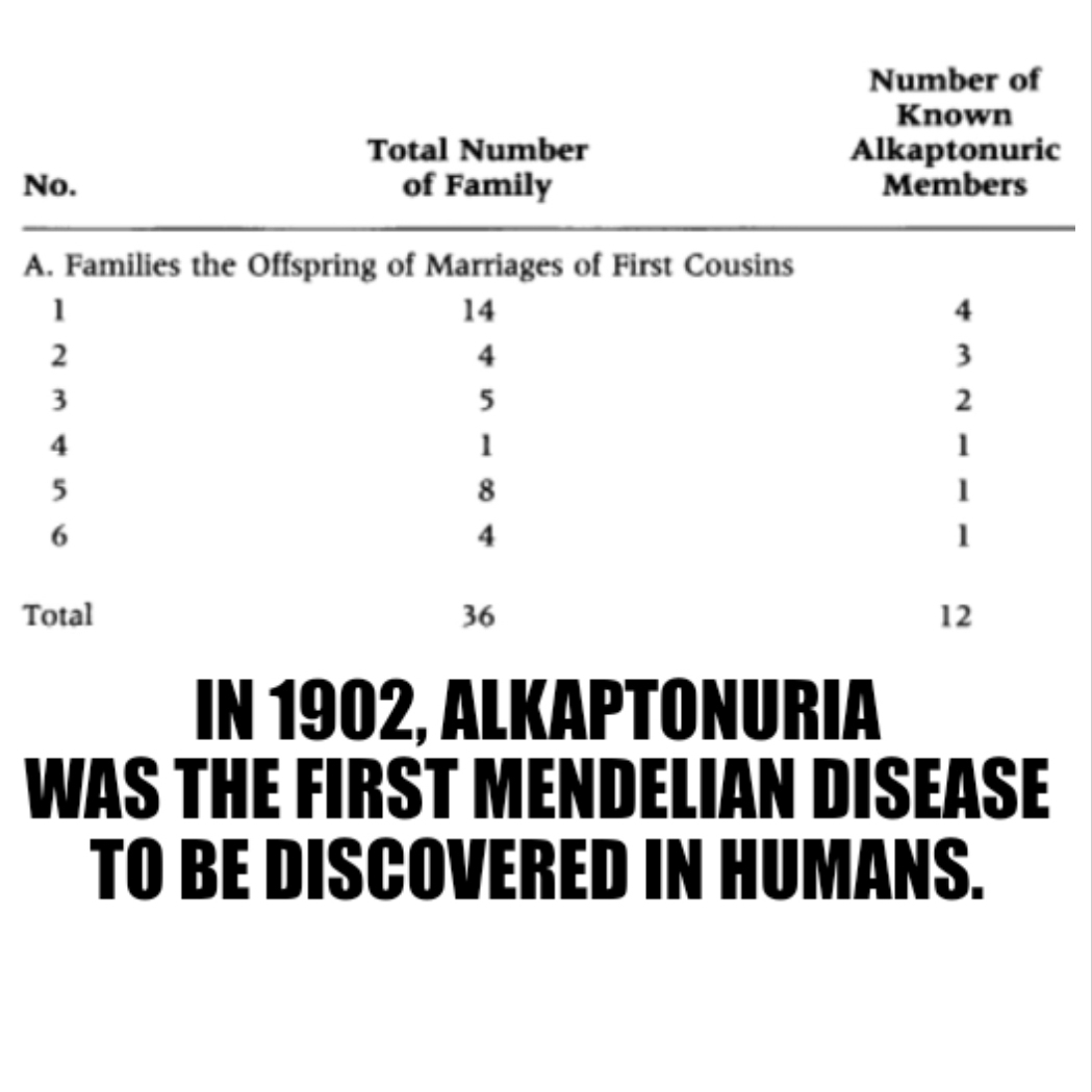
Garrod noted to his friend Bateson that this disease was found most often as the result of marriages between first cousins, and at Bateson’s urging, Garrod documented the incidence of Alkaptonuria in these families.
Today’s #FigureFriday is the first evidence of a recessive Mendelian disease in Humans.
In the table you can see that in these families the dominant form of the trait is observed in 36 offspring, and the Alkaptonuria form in 12.
This perfectly aligns with the 3:1 ratio Mendel first observed in his peas!
###
Garrod AE. 1902. The incidence of alkaptonuria: a study in chemical individuality. The Lancet. DOI: 10.1016/S0140-6736(01)41972-6
2
5
984
27 Jul 2023
Detecting variants can be challenging, especially detecting the ones that aren't very abundant.
Unfortunately, there are a good number of labs that use the default settings for their sequencing analyses, and/or implement premade pipelines that they 'validate' without doing the appropriate amount of work to make sure that the thing they've developed actually performs the way they say it does.
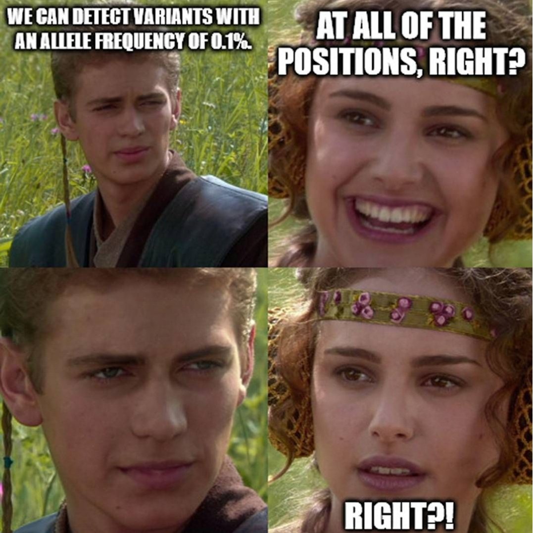
This gets extra tricky in oncology screening where the allele frequencies can drop well below 1% with the latest crop of sequencing based tests advertising sub 0.1% detection capabilities.
But what does it mean to be able to call a heterozygous variant with a 50% frequency in a germline sample or a 0.1% frequency variant in a liquid biopsy?
Can the assay do it everytime time?
Can the assay do it in every sequence context?
How do you know?
There are a few really good ways to know, but most places don't do these things because they're not required to:
In silico decimation - this is an informatic technique where the data from a large number of samples is randomly reduced ie take samples with a minimum coverage of 40x at each position and reduce them to 30x, 20x, 10x to see where the assay starts losing the ability to detect specific types of variants. In the case of liquid biopsy samples where the minimum coverage to call a sub 1% variant approaches 10,000x (depending on the quality/error correction strategy), decimation through a much higher coverage range might be warranted. It is also possible to create contrived datasets where variants are randomly inserted into the data at a specific frequency, but these programmatic manipulations of frequencies are only good for evaluating informatics performance, not lab process performance.
Contrived synthetic controls - one way to test process performance is to synthesize a variant into a sequence using a company like Integrated DNA Technologies and then spiking or diluting that sequence fragment into a sample to 'contrive' the mutation. This 'sample' can then be taken through the whole process and be used to determine at what allele frequency the lab process begins to fail to detect the variant (preferably this is done for every gene/target/exon in the panel).
Characterized mixture panels - many companies (and NIST) offer mixture panels. Some are contrived, others are mixtures of cell lines with well known variants, but most importantly, these panels have been independently characterized using sequencing and/or droplet PCR to precisely determine the allele frequencies of the variants contained in the panels. These allow for accurate benchmarking of the performance of an assay using an independent resource.
However, none of these methods is perfect and it's always a good idea for labs to track assay performance post-launch, especially as interesting positive samples are gathered or become available through other sources.
2
6
21
3,143
26 Jul 2023
This paper is low key mindblowing and it got 7 likes and 3 retweets 🤣 Review coming next Tuesday.
19 Jul 2023

Analysis of #plasma #proteomes of 1477 patients across twelve cancer types and machine learning lead to a protein panel for cancer classification
#CancerResearch by @_buenoalvez @ProteinAtlas
@NatResCancer
nature.com/articles/s41467-0…
3
323
25 Jul 2023
Spoiler Alert: The future of disease early detection isn't going to be genomics.
We already have some pretty good hints that this is true.
One of them is that the hottest Multi-cancer early detection (MCED) screening test is based on methylation.
This falls squarely in the realm of epigenomics.
But we also have three decades worth of high throughput genomics under our belts now and we really don't have a ton to show for it.
We've certainly learned a lot in that time about the genome but one of the greatest lessons we've been taught is that genetics alone is a pretty terrible predictor of whether a healthy person will actually develop a disease.
Recent studies have shown that 8% of people carry a pathogenic mutation, but only about 7% of those people ever become symptomatic.
The caveat here being that some mutations are more likely to cause disease than others. These include mutations in BRCA1 and BRCA2 (Breast Cancer) or HBB (Thalassemia) in which 30-60% of patients with those develop disease.
But what do we do with all of the other 'damaging' pathogenic variants we find in healthy people?
The American College of Medical Genetics (ACMG) suggests extending the list of reportable findings to include pathogenic variants in 81 disease associated genes (inclusive of the 3 above).
These are all considered to be 'medically actionable' because steps can be taken to improve their clinical outcomes.
However, the struggle here, and with most genetic diseases, is knowing when, or if, a healthy person will ever become symptomatic.
Wouldn't it be great if we had a way to detect disease onset decades before there's an observable phenotype in a patient?
We're finally at a point where this might be possible and it's all thanks to new developments in proteomics (the study of proteins and how they interact within our cells)!
Interest in proteomics has increased drastically in the past few years as new technologies have made it possible to easily study thousands of proteins at a time in a single sample.
The power of these methods was highlighted in a recent paper where an aptamer array was used to screen ~5,000 proteins in the plasma of 11,000 patients who had participated in a 25-year study on atherosclerosis.
The researchers were able to use blood samples collected throughout the duration of that original study to identify a set of proteins that could predict the development of dementia up to 25 years before symptom onset.
That's pretty incredible!
While there's still a lot of work to be done, it's exciting to see how proteomics continues to increase our understanding of the biology of disease.
Because, as we've learned, the genome only represents potential, but the proteome could tell us when, or if, that potential is actually beginning to impact biology!
###
Walker KA et al. 2023. Proteomics analysis of plasma from middle-aged adults identifies protein markers of dementia risk in later life. Sci Transl Med. DOI: 10.1126/scitranslmed.adf5681
5
13
1,869
Brian Krueger, PhD retweeted

23 Jul 2023
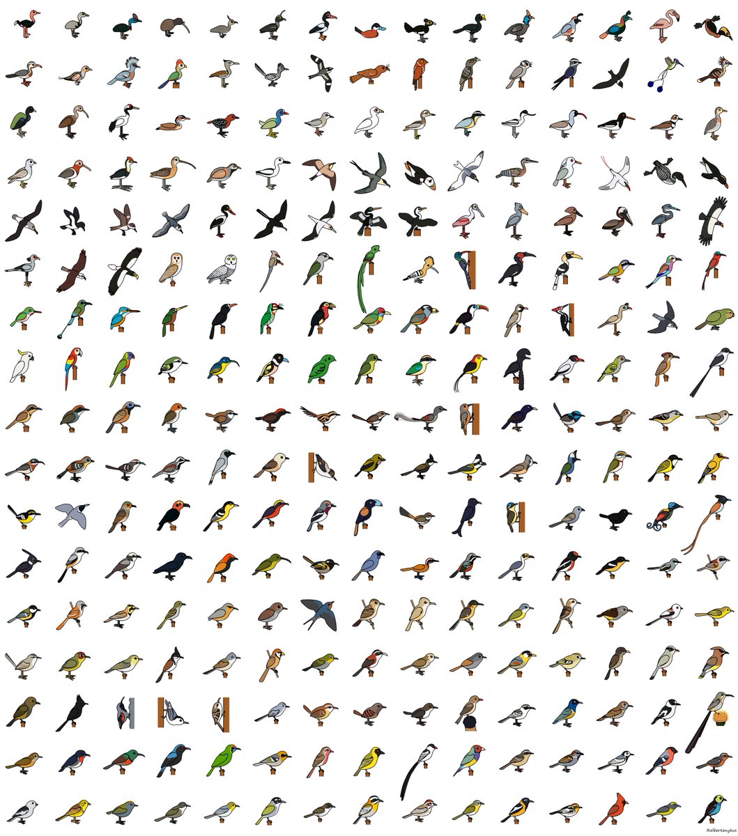
A wise artist once said, "Any reason is a good reason to draw a [bunch of] birds." I've now drawn a representative of every living bird group ranked at the level of family by the IOC World Bird List (and a few that aren't)!
13
257
1,310
88,179
21 Jul 2023
The two gels below spawned a multi-billion dollar industry that didn't exist prior to their publication in 1997.
While it may seem obvious today, you might find it surprising that we didn't know that fetal DNA was present in a pregnant mother's bloodstream until the late 1990's.
Prior to this discovery, genetic testing on fetuses was only performed if a problem was suspected with a pregnancy or if there was a family history of genetic disorders.
This testing was performed by karyotyping fetal cells.
You've probably seen one of these 'chromosome spreads' in a biology textbook where each of the 23 pairs of chromosomes are lined up next to one another.
This allows a geneticist to check that the chromosomes are intact and see if there are any abnormalities such as those found in Down Syndrome where patients have 3 copies of chromosome 21 instead of 2.
But, back in 1997, the process for collecting fetal cells was very invasive and was done using one of two techniques:
Amniocentesis (Amnio) - a 3-5" long needle is inserted into the mother's abdomen to collect 20 milliliters of amniotic fluid for testing.
Chorionic Villus Sampling (CVS) - A 6" long needle is guided via ultrasound, either vaginally or through the abdomen, to obtain tissue from the placenta for testing.
Unfortunately, these procedures carry a risk and could lead to the loss of the fetus in 1-2% of the procedures.
Recognizing that there had to be a better way, Yuk-Ming Dennis Lo set about figuring out how to get at fetal DNA without having to perform Amnio or CVS.
He knew that fetal cells made it into the maternal bloodstream and that mother and child exchanged cellular material but he couldn't isolate enough fetal cells from the blood to do prenatal genetics with them.
Luckily, in 1996, Lo heard that a team in Switzerland had shown that tumors actually shed cell free DNA into the bloodstream and this tumor DNA could be detected using PCR and primers specific to the tumor DNA.
He reasoned that a baby, or more accurately, the placenta, was basically like a giant tumor and shared the bloodstream with the mother and so it made sense that it too should shed cell free DNA into the bloodstream.
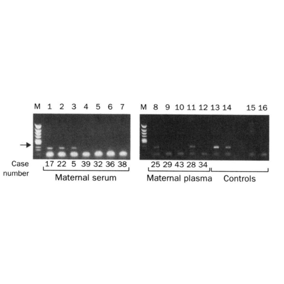
Today's #FigureFriday is proof that Lo's hypothesis was correct and fetal DNA could be isolated from the blood of pregnant females and amplified using PCR.
In this figure, the arrow highlights a 198bp PCR product from the Y chromosome. Case numbers greater than 30 are pregnancies with female fetuses (don't have a Y), and case numbers less than 30 are male fetuses (have a Y).
Further technical advancements and the invention of high throughput sequencers in the early 2000's have transformed this discovery into a popular pregnancy screening test.
Today, non-invasive prenatal testing is second only to oncology applications in sequencing market share.
###
Lo YMD, et al. 1997. Presence of fetal DNA in maternal plasma and serum. The Lancet 350(9076), 485–487. DOI:10.1016/s0140-6736(97)02174-0
2
32
133
20,500
20 Jul 2023
High throughput sequencing:
Biases and how they can get the best of you and your data.
One thing that has always kept me up at night is thinking about all of the different ways that bias can be introduced into the genetic testing process.
Nearly every step presents multiple opportunities for the results to be inadvertently altered.
Bias is especially problematic in diagnostic testing and an inordinate amount of effort is expended to reduce or eliminate these biases in every step of the process.
This is because getting an answer wrong, or missing a diagnosis, has an immediate negative impact on a patient.
So what are some important sources of bias in genetic testing?
Sample Collection - This one can be tricky, especially in oncology and infectious disease because getting 'enough' or sampling the right location or region of the tissue can mean the difference between detecting the disease or infection or missing it completely. In the case of germline genetics, blood is the best and least biased source, while oral swabs and spit are potentially the most biased since your mouth is full of bacteria and, depending on the test method, this can reduce the overall quality or coverage of the final result.
Shipping/Transport - Making sure the sample gets to the testing site without degrading is a big deal. This is usually accomplished by keeping the samples cold or stabilizing them in a solution that prevents degradation of the DNA or RNA in the sample.
Nucleic Acid Extraction - The process in which you liberate the nucleic acid from cells can be a significant contributor to bias. Not all cells behave entirely the same way and this is especially true when extracting nucleic acid from bacteria, some of whom have a hard candy shell that requires a little extra oomph to be sure you get it all out in an unbiased way.
Fragmentation/Library Preparation - There are many 'easy' or 'rapid' kits on the market that introduce a substantial amount of bias into your libraries. It is important to understand the benefits and limitations of the enzymes used in each of the available methods.
Target Capture - Probe hybridization and capture is an inherently biased process because the efficiency of binding and capture is highly dependent on the sequence content of the region being targeted.
GCbias - This occurs as a result of PCR amplification during the library preparation process. GC base pairs have 3 hydrogen bonds while AT pairs only have 2. PCR is biased against regions with high GC because it takes more time to push apart 3 bonds. One thing that is rarely talked about is how much less biased single molecule methods (long-reads) are than cluster based methods (short-reads). Clustering is essentially an amplification step and so will always suffer some level of bias against high GC regions.
Reference Genome/Variant Databases - Most cater to a European ancestry. This currently makes it somewhat challenging to make informed decisions in non-white populations.
2
3
9
2,887
19 Jul 2023
Crane, pheasant, peacock? Nope, that's a Hoatzin, and no one really knows where it came from.
If we've learned anything from the history of science, some of our best lessons in genetics come from studying plants and animals.
Birds are an especially useful subject for these sorts of studies because, typically, they have distinct physical characteristics.
Even Charles Darwin famously wrote 'On the Origin of Species' after an expedition to the Galapagos where he studied the beaks of finches (a small bird) and developed what we now think of as modern evolutionary biology.
A big part of Darwin's theory being that beneficial traits are selected naturally, and those that confer an advantage to an individual are passed on to their offspring.
Those individuals are then said to increase their 'fitness,' which is a measure of reproductive success - more reproduction equals better fitness.
So that means that traits are inherited and we can figure out the ancestral history of animals by successively grouping the ones that look alike together.
At least that was the thinking in the mid-1800's.
This ends up more or less becoming a tree where every branch has a distinct common ancestor and the things that all look alike are related.
But, unfortunately, biology isn't that simple, nor is evolution.
Because what's beneficial to one group or individual could be beneficial to another. And instead of inheriting a trait from an ancestor, two groups can develop that same trait independently of one another.
There are many examples of this evolutionary process in action, a classic example of this being wings in bats, birds and insects.
These are totally different animals who all evolved the ability to fly separately, but this developmental agreement on similar physical structures is called convergent evolution.
While these things might look the same on the physical level, they're totally different on the molecular and genetic level!
Fortunately, DNA sequencing can help suss out what's inherited and what's convergent, but in the case of the hoatzin, it's not so simple.
Actually, all modern birds aren't so simple once we look at the genetics.
It might seem easy to stick something that looks as weird as the Hoatzin off on its own, and group modern birds nicely into evolutionary branches based on their physical characteristics.
But that's not what DNA sequencing tells us and modern birds seem to have hybridized so much that their evolutionary origins actually look a lot more like a network, or a bush, than they do a typical tree!
Even the Hoatzin, which by all accounts should be stuck in a corner by itself, has genetic signatures that make its origins not totally obvious.
It would seem that our view on evolutionary trees also needs to evolve.
###
Suh A. 2016. "The phylogenomic forest of bird trees contains a hard polytomy at the root of Neoaves." DOI:10.1111/zsc.12213
1
2
232
14 Jul 2023
The structure of the DNA double-helix was published in 1953, but it took another 13 years to actually crack the genetic code.
The two key questions after the structure of DNA was figured out were:
1) How is it copied?
2) How does it code for proteins?
The first question was answered by Meselson and Stahl in 1958. DNA is copied ‘semi-conservatively’ - the old strands serve as a template for creating the new complementary strands.
The second question wasn’t fully resolved until 1966.
There, of course, were theories about how this occurred and Francis Crick gave a seminal lecture in 1957 (published as a paper in 1958), ‘On Protein Synthesis,’ which laid out the basic formula for how he believed this all worked.
He got it mostly right.
He proposed that there must be an 'adaptor' which carries the amino acids (we now call this transfer RNA, tRNA) to the template RNA (this became messenger RNA, mRNA) to synthesize the protein chain.
But Crick also hypothesized in this lecture that the genetic code is read 3 nucleotides at a time.
It was known that there were 20 amino acids and so Crick reasoned that since there are only 4 nucleotides in DNA and RNA, the ‘code’ for each amino acid couldn’t be 2 nucleotides (4x4) because that’s only 16 combinations, so optimally, it was a 3 nucleotide code (4x4x4) because that combination gave 64 possibilities - ~3 combinations for each of the 20 amino acids.
The first indication that Crick’s hypothesis was true came in 1961 when Nirenberg and Matthaei showed that an RNA sequence containing only U’s coded for poly-phenylalanine.
Inspired by this result, Crick showed that insertion or deletion of 1 or 2 bases causes proteins to become non-functional, but 3 base mutants still produce functional protein.
The code must be a triplet!
Nirenberg and Leder followed up in 1964 with triplet codes for a handful of amino acids but they frustratingly couldn't determine all of them.
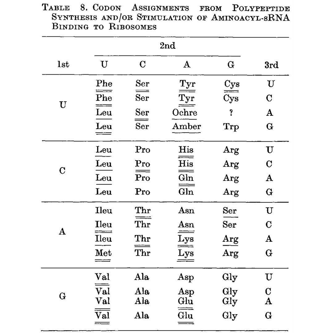
That problem was solved by Har Gobind Khorana, an Indian American scientist, whose work is the subject of this #FigureFriday.
While Nirenberg and team were using binding assays to try to capture the RNA-amino acid associations, Khorana approached it differently by synthesizing repeating dinucleotide and trinucleotide RNA polymers and seeing which amino acids ended up linked together in the resulting protein chain.
The outcome of this work can be seen below (underlines), and this is the first presentation of a nearly complete codon table. The only missing assignment is UGA, the third and final stop codon.
Unsurprisingly, Khorana, Nirenberg and Holley (he determined the structure of tRNA) shared the Nobel Prize in 1968 for deciphering how nucleic acids code for proteins.
###
Khorana HG, et al. 1966. Polynucleotide Synthesis and the Genetic Code. Cold Spring Harbor Symposia on Quantitative Biology, 31(0), 39–49. DOI:10.1101/sqb.1966.031.01.010
7
34
4,485
13 Jul 2023
High throughput sequencing metrics:
Q-scores, what are they good for?
If you've done sequencing in the last 30 years, you've heard of a Q-Score and you probably know that they're a measure of quality.
But what you might not know is where this metric came from.
The idea of base quality scores emerged in the early 1990's as a result of the automation of Sanger sequencing.
These new systems used fluorescent dye terminators instead of radioactively labeled ones.
This meant that instead of looking at bands on a gel to determine the sequence, scientists now analyzed fluorescence and so a program called 'Phred' was developed to make accurate base calls from the fluorescence intensity plots.
But a huge advancement in Phred was the inclusion of a quality score for each base call that it made.
We lovingly refer to these today as Q-scores!
These Q-scores are a log based estimation of the quality of the call.
Phred determined this originally based on an error estimation that took into account the peak height and shape of the fluorescence 'trace' for each base.
Today, these scores are calculated somewhat similarly in that they're still the log of an error estimation, but the factors that go into that estimation can be quite complicated!
The Q-scores we deal with most frequently range from 10-50 and they have the following accuracies:
Q10 - 90%
Q20 - 99%
Q30 - 99.9%
Q40 - 99.99%
Q50 - 99.999%
'So is there a benefit to having a higher Q-score or are they just a marketing scam?'
That's complicated.
They're not a scam since most pipelines Q20 or Q30 trim their base calls to be sure that only bases with a quality of >99% make it into downstream analysis.
'But is there a difference in the usefulness of a Q50 dataset over a Q20 dataset?'
It really depends on the application.
Something we hear about constantly in the whole genome sequencing space is the need for 30x coverage for us to make heterozygous (het) variant calls.
This is important because, if you remember, your genome is composed of two copies of DNA: one from your mom and the other from your dad.
So every position in your genome can be homozygous (same sequence from both parents) or heterozygous (different sequence from each parent).
Interestingly, sampling statistics (math) say that to be >99% certain of a heterozygous base call, you need to look at each position in the genome 30 times.
But even more interestingly, if you look at plots of variant call accuracy vs coverage for Q20, Q30, or Q40 data, they all converge on ~30x coverage for >99% het variant calling!
'So it is a scam!!!'
No, it's just math.
There are applications where higher quality bases are useful, especially in oncology or therapeutics where the variants you care about aren't at frequencies of 50% and 100%, but sub 1% or even lower.
Here, Q40 (99.99%) or Q50 (99.999%) really shine because then the error of the base calls isn't fighting with the frequency of the variants!
3
14
53
8,816
7 Jul 2023
A and T, and G and C are present in the same amounts in DNA. It’s like the most basic rule of DNA. It’s also called Chargaff’s Rule.
Well before the structure of the DNA double helix was revealed by Watson and Crick (with the help of Rosalind Franklin!), biochemists first had to figure out the chemical make-up of deoxyribonucleic acid.
Identifying the bases and how they were linked together with a phosphate backbone was the work of Phoebus Levene. He was the first to tease out the chemical makeup of ‘desoxypentose nucleic acid,’ which we lovingly refer to today as DNA!
However, because only 4 bases existed, Levene triumphantly declared that DNA was far too simple to be considered as the chemical that stored the genetic information of organisms.
He fell into the same trap as most everyone else at the time, and believed that protein was the genetic material.
Levene proposed the ‘tetranucleotide hypothesis’ which stated that DNA was made up of repeats of the same 4 nucleotides and these nucleotides were present in equal amounts.
We now know that this was totally wrong and part of the reason why Levene thought that nucleotides were present in equal amounts was because the analytical methods used in 1928 were not accurate enough.
It took another 22 years, and the invention of much more sensitive paper based chromatography techniques to tease out the true chemical nature of DNA.
But the first cracks in the hypothesis that ‘proteins are the genetic material’ appeared in 1944 when Oswald Avery, Colin Macleod and Maclyn McCarty showed in a series of experiments that DNA, and not protein, could ‘transform’ the bacteria pneumococcus.
While the majority of scientists at the time ignored this paper, because the results were contrary to popular belief, Erwin Chargaff of Columbia University was intrigued.
He saw Avery’s results as the first evidence that maybe the field had it all wrong about DNA, and that it wasn’t just a random jumble of nucleotides but something much more important.
So he did what he did best, got in the lab, extracted a bunch of DNA from a bunch of different organisms and calculated in exacting detail how much of each base was present in every sample he tested.
A good number of these papers are in German, but the one that I’m pulling from today was published in Nature in 1950.
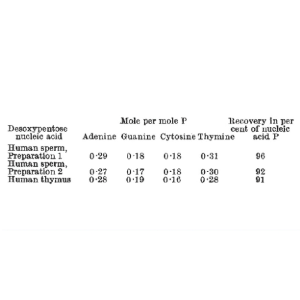
Today’s #FigureFriday is a table showing the nucleotide content of human sperm and human thymus.
~28% of human DNA is made up of Adenine, 18% Guanine, 18% Cytosine, and 30% Thymine. These results show that the nucleotides aren’t all present in the same amounts as Levene had hypothesized, but that Adenine and Thymine, and Guanine and Cytosine are found in equal concentrations.
This was a key discovery on the path to showing how these seemingly complementary nucleotides bound together in the structure of DNA.
###
Chargaff E, Zamenhof S, Green C. 1950. Composition of human desoxypentose nucleic acid. Nature. 165 (4202):756–7. DOI:10.1038/165756b0
1
3
3
1,083
6 Jul 2023
High throughput sequencing metrics:
Let’s be accurate about accuracy.
If “What is a genome?” is the most loaded question in the world of short-reads, the most loaded question for long-reads is “What’s the accuracy?”
A lot of this comes down to the semantics that PacBio and Oxford Nanopore (ONT) use when talking about accuracy.
Because in conversations they tend to use the different types of accuracy essentially interchangeably.
There are 3 main types of accuracy in sequencing:
Base Accuracy - The accuracy of each individual base call. This is the traditional Phred Q-score and a general measure of quality used for assessing most short-read sequencing outputs. Element is Q40 (99.99%), Illumina/Complete is Q30 (99.9%), and Thermo is Q20 (99%).
Read Accuracy - Up one level from base accuracy, what percentage of the bases in a read are accurate. PacBio HiFi reads are 99.9-99.999% accurate, ONT is 70-99.9% accurate.
Consensus Accuracy - The accuracy of the consensus sequence, or, the accuracy after assembling all of the data using multiple reads to correct all the errors.
Before PacBio released HiFi reads, both PacBio and ONT required 'polishing' to produce useful datasets. Reads where ~25% of the bases are wrong are challenging to use for most sequencing applications.
Polishing requires the use of short reads to correct all of the errors because of their very high accuracy, and so long-reads struggled to gain traction beyond niche genome scaffolding applications since these hybrid sequencing approaches are very expensive.
Another expensive method for correcting these sorts of errors is to just do more sequencing.
This works for PacBio because the errors in their data are random. This is why HiFi circular consensus sequencing (CCS) has such high read accuracy, it’s a self-polishing method!
It also works for some ONT data errors, but their method is prone to systematic errors (always happen in the same sequences), so sequencing more will not remove those and requires short-read polishing methods to be fully resolved.
More recently, ONT have touted read accuracies at the same level as PacBio, with sequences for HG002 coming off their dual reader R10 pores with a 'duplex' read accuracy of 99.9% .
But, at the end of the day, the key thing to know about accuracy is that traditional base accuracy is more relevant for short-reads when addressing quality and read accuracy and consensus accuracy are more important for long-reads.
This will become more apparent as each of the two technologies settle on the niches where they excel - long-reads for high quality genomes, and short-reads for just about everything else!
2
6
6
1,381
Brian Krueger, PhD retweeted

Why is it that the people who cut corners always whine the loudest about regulation stifling innovation?
You might have heard that a submarine imploded recently while on a luxury tour of the site where the Titanic sank.
Ok, maybe not luxury, but a very expensive tour of the Titanic, because anyone with two functioning neurons who looked at the OceanGate Titan might question why a ticket for such a voyage would cost $250,000 when the 'submarine' appeared to be held together with bubble gum and bailing wire.
Things got worse on the inside where the 'craft' was controlled by a $40 Logitech gamepad.
Despite its 4-star review on Amazon, the most significant problem with this sub wasn't the gamepad, but the materials hiding just outside of view that were used to create the pressure hull of the Titan.
Now, pressure hulls of most deep submersion vehicles (DSVs) are spherical and made out of titanium, aluminum or steel.
Basically every deep dive record is held by a DSV built around a titanium bathysphere.
The Triton was different, it was cylindrical in shape.
It was also made out of a combination of titanium, carbon fiber, and acrylic.
Despite being warned that a carbon fiber and titanium composite hull was basically a ticking time bomb, Stockton Rush, an aerospace engineer and CEO of OceanGate, continued to take the Titan to depth until it imploded after a handful of dives with 4 paying customers onboard.
You see, marine engineers saw problems with Titan's design and the materials that were used in its construction.
Notably, carbon fiber isn't a great choice for pressure hulls because it's much less tolerant of compressive forces than tensive ones.
So, while carbon fiber might be a great choice for aerospace applications, it's a terrible one for a pressure hull.
Carbon fiber subjected to repetitive cycles of compression can fail unexpectedly and although Rush was warned that it was only a matter of time until his sub had a catastrophic failure, he instead sold paying customers trips on a sub that he said was safe.
In an interview with David Pogue at CBS, Rush said, "the part that keeps you alive, the part we care about, is that carbon fiber cylinder and the titanium end caps [which were] buttoned down."
The problem here is that Rush was the only one that thought any of this was true and duped customers, unknowingly, into playing a very high stakes game of Russian roulette.
Rush once said that 'obscenely safe' regulations had been holding back his 'innovations' for years, but refused to submit any of those innovations for testing and certification.
Unfortunately, it took the deaths of 5 people to remind us why regulations exist and why it's so important to prove empirically the performance, efficacy, and safety of the thing you developed before releasing it publicly.
That's true for subs, but also automobiles, airplanes, medical devices, drugs or any other product whose use can result in serious injury or death.

2
3
762