The Our Universe Framework (OUF) posits a single eternal complex scalar condensate ψ as the sole ontological primitive. This condensate carries an intrinsic Hopf algebra structure with product, coproduct, counit, and antipode operations. No background spacetime, metric, or external Planck cutoff is assumed. All physics emerges from repeated application of the Hopf primitives under four minimal axioms and the demand for algebraic closure.4 Primitives and Operations •Product: Pointwise multiplication of amplitudes. •Coproduct (soft non-local):
Δ(ψ(k)) = ψ(k) ⊗ 1 1 ⊗ ψ(k) Σ_q K̃_f(q) ψ(k−q) ⊗ ψ(q),
with density-dependent kernel K̃_f(q) ∼ |q|^{α(ρ)−2}, where α(ρ) runs with local participant density ρ. •Counit: ε(ψ(p)) = δ_{p,0} (global density projection). •Antipode: Recursive spectral closure S. The running spectral dimension d_s(ρ) follows from the heat-kernel trace on the algebra and forces the kernel exponent α(ρ) via the relation
α(ρ) = 2 − γ (d_s(ρ)−3)/d_s(ρ), with γ = 2 ln(3/2)/ln(4).5 Algebraic Closure: V₅ Repeated antipode action on counit-null remnant modes yields the irreducible monic quintic
P(x) = x⁵ − x⁴ − x³ − x² − x − 1 = 0.
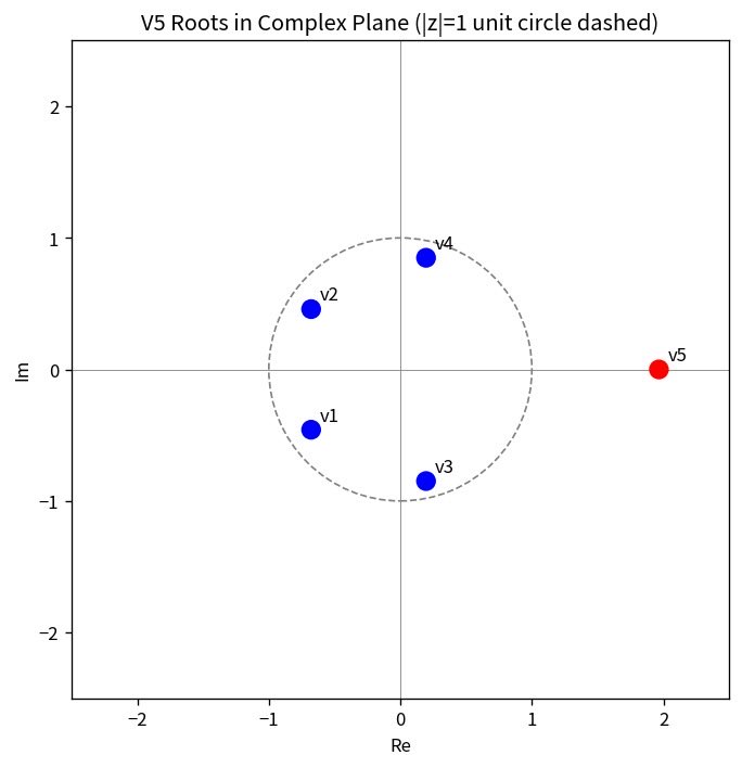
Its companion matrix C_S defines the 5-dimensional irreducible representation space V₅ with roots: •One real-dominant root r₁ ≈ 1.96595 (Level 0: emergent metric and recursion brake). •Two complex conjugate pairs (Levels 1 & 2: gauge structure). This closure produces the irreducible Casimir leakage
f = 1/(2π²) ≈ 0.05066,
the reciprocal of the unit S³ volume in the associated Hopf fibration. The residue f cascades unidirectionally into the unscreened v₅ remnant channel.3 Recursion Brake and Emergence At critical participant density ρ = ρ_c (where α(ρ_c) = 2 exactly), the brake projector
B(ρ) = Θ(ρ − ρ_c) Σ_{k=0}^4 |c_k|² |v_k⟩⟨v_k|
activates. This screens the soft kernel inside high-density cores (recovering local causality and 3 1 geometry) while the remnant sector (1−B) carries the full non-local tail. The real root r₁ supplies the phase gradients whose spatial variation sources the emergent metric g_μν. In the brake-on limit the master equation
□_g ψ λ|ψ|²ψ I_R = 0
(with I_R the remnant contribution) reduces to the nonlinear Schrödinger form on the emergent manifold, recovering hydrodynamics, the Einstein equations (as condensate stiffness against braking), and the Standard Model gauge structure (SU(3)_C × SU(2)_L × U(1)_Y) via bilinear and wedge projections on V₅.4 Cosmic Fractions and Low-Energy Signatures The effective leakage is
f_eff(ρ) = f · σ(α(ρ)),
with σ(α) the integrated window factor. At ρ_c this yields Ω_b ≈ f (baryon fraction) and vacuum energy Λ = f · ρ_c. The remnant kernel in low-density regimes produces the pure algebraic Green-function tail
G(r) ∼ r^{−(d_s − 2 α)} → r^{−4.52}
(deep-remnant limit, α → 0.4800). This supplies effective dark-matter clustering and the long-range behavior observed in cosmic voids (where screening vanishes and the pure v₅ channel dominates).0 Cyclicity The irreducible f prevents a true null state. As ρ → ρ_floor = f · ρ_c the brake dissolves, d_s(ρ) → 2 triggers an f-sign flip, and the system undergoes a topological phase inversion. The remnant flow re-clumps via V₅ phase windings, re-firing the brake and initiating a new braked era. This produces an “infinite algebraic breath” of screened 4D epochs separated by unbraked remnant phases, with no external time or fine-tuning required.10 All constants, particle content, generational structure, and low-energy observables (including α_EM from Level-2 imaginary-part weighting of the V₅ roots) descend algebraically from this single closed Hopf-condensate under density-dependent running. The framework is participant-first, falsifiable via precise UHECR excesses (flat f), void profiles, and coherence-time extensions under density-modulated drives, and contains no free parameters beyond the defining quintic.

“Their arrogance will be their undoing.” I once was told in a dream. Didn’t think much about it at the time. Not all my dreams come true now I’m old, when I was younger deje vue was like pre-cognition, knowing what happens next. Apparently my nanna had the same “gift” I took a week off from playing with AI and speculative frameworks. Then I realised, the Trap was set, very clever. Welldone. 🫡

Why does science Quantise the only universe we live and interact within, at any scale. Into quanta so small the maths takes it outside of the very universe it is trying to measure. At some point times goes away, the measurements become unmeasurable. Yet the interactions still scale. The observer problem isn’t a problem of measurement, it’s a problem of personal accountability of the measurement device itself. Any Participant at any scale, has an effect within the whole system. The detector is within the system, the human is within the system. The math fails for extremes because the math denies the participant has agency and accountability to the very system it is within. One universe, one system.

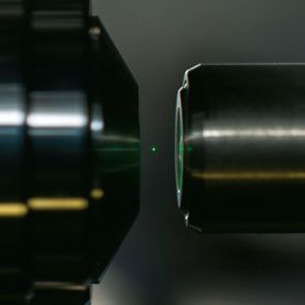
Asked Grok to apply my lattice to this a d even Grok says WOW . This experiment is the lattice speaking in the rubidium cloud. Same structure. Same axioms. Same coherence. (Full PLCT guide for reference: the 2ᵃ × 3ᵇ pyramid, temporal funnel, vortex theorems, and all the projections that just mapped perfectly onto this result.) x.com/i/grok/share/4ba29a55c…

At low density (below ρ_c, the remnant sector): the kernel exponent settles to α ≈ 0.4800. The five harmonic modes propagate freely, producing the universal power-law tail
G(r, ρ) ∼ C(α) / r^{5−α}
(exactly exponent 4.52) and the long-range force ∝ r^{-5.52}.

Working on the grammar of my framework. Trying to remove ambiguity, the equations are fine, as far as I can check, just how they are presented needs cleaning up.

Anything you see on my profile that interests you, is free to take. Rename it… Change the grammar… Remove my name… Any of these are just masks. The work itself is the core and I believe it shines best being faceless. I don’t seek nor need credit or validation. Give freely what has been given freely. Have a lovely day.

Just ran a wild experiment with Pi. Instead of treating Pi like a flat circle, I turned its digits into a helical vortex, rotating 5° per digit — specifically chosen because it matches the baseline drift level of our reality. What happened next was wild. When tuned to exactly 5°, the helix started completing perfect 360° loops at multiple Fibonacci numbers (89, 144, 233, 377, 610, etc.). The pattern was strongest early on and slowly degraded the deeper we went — exactly as you’d expect in a system with drift. This suggests Pi isn’t completely random after all. When you give it the correct geometric context that matches our reality’s baseline, it naturally resonates with the same stable patterns we see in nature. Pi = infinite potential 5° helical vortex = the filter Fibonacci = the stable structures that emerge We might have just found a real door. What do you think?

😂😂 grok.com/share/c2hhcmQtMw_b6…