
Joined April 2023
- Tweets 2,435
- Following 28
- Followers 63
- Likes 3
20 Photos and videos


🔍 A confusion matrix helps evaluate model performance, linking directly to metrics like accuracy, precision, recall, and F1 score.
Understanding these concepts enhances your ability to fine-tune models and improve predictions!
1
5
🌐 Sphericity is a key concept in statistics, especially in repeated measures ANOVA.
It checks if the variances of differences between groups are equal.
This helps ensure accurate results!
4
📊 Embrace the power of boxplots!
They reveal not just data distributions but also hidden outliers—those unique insights that can drive innovation.
Remember, sometimes the outlier is the breakthrough waiting to be discovered!
1
31
📊 Always visualize your residuals!
Plotting them against fitted values can quickly reveal violations of homoscedasticity.
If you see patterns, consider transformations or robust methods to improve your model.
8
📊 In a recent project, I used stratified sampling to analyze customer feedback.
By dividing respondents into age groups, I ensured each segment was represented, leading to more accurate insights.
This helped tailor marketing strategies effectively!
1
4
📊 A histogram is a great tool for checking if your data is normally distributed!
It shows the frequency of data points in different ranges.
Look for a bell-shaped curve.
If it’s bell-shaped, your data is likely normal!
1
6
🧠 Remember: population parameters are true values for the entire group, while sample statistics are estimates from a smaller subset.
Always use sample stats to infer about the population, but be mindful of sampling bias!
1
5
🔍 Fisher's exact test is invaluable for analyzing small sample sizes in categorical data.
Use it to assess the association between two binary variables, like treatment success vs.
failure.
Implement it in R with `fisher.test()`!
1
7
🌟 To improve classification accuracy, always start with data preprocessing.
Clean your data, handle missing values, and standardize features.
A well-prepared dataset leads to better model performance!
1
4
🔍 Ensure your residuals exhibit homoscedasticity for valid statistical inferences.
Use residual plots to check for constant variance; if not, consider transformations or robust methods to improve your model.
1
4
📊 A boxplot shows data distribution with a box for the middle 50%, lines for min/max values, and dots for outliers.
Outliers are values much higher or lower than most.
They help us spot unusual data points!
1
4
📊 In a retail analysis project, using advertising spend (independent variable) to predict sales revenue (dependent variable) can guide budget allocation, boosting profits.
Effective data-driven decisions can transform business outcomes!
1
5
📊 Kendall correlation is a powerful tool for non-parametric data, measuring ordinal associations without assuming normality.
It's essential for robust statistical analysis, especially in fields with ranked data.
1
7
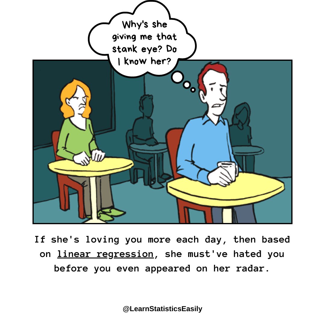
📊 Aim for a sample size of at least 10-15 observations per predictor variable in linear regression to ensure reliable estimates and reduce variability.
This helps in achieving robust and generalizable results.
1
6
✨ In the realm of data, random samples capture the chaos of reality, while systematic samples unveil hidden patterns.
Both methods are keys to unlocking insights—balance them to illuminate the unseen!
1
8
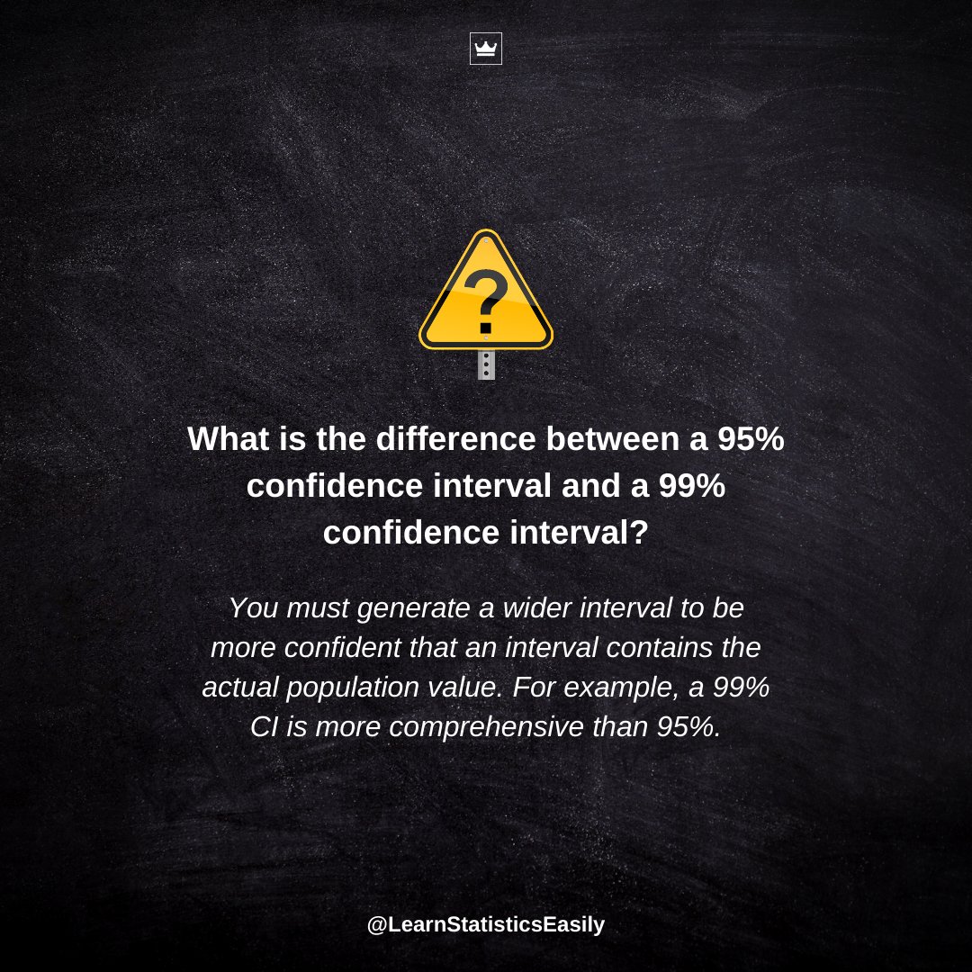
📊 Confidence levels (90%, 95%, 99%) help quantify uncertainty in estimates.
Use them in hypothesis testing and interval estimation.
For example, a 95% CI for a mean gives a range where we expect the true mean to lie.
1
5
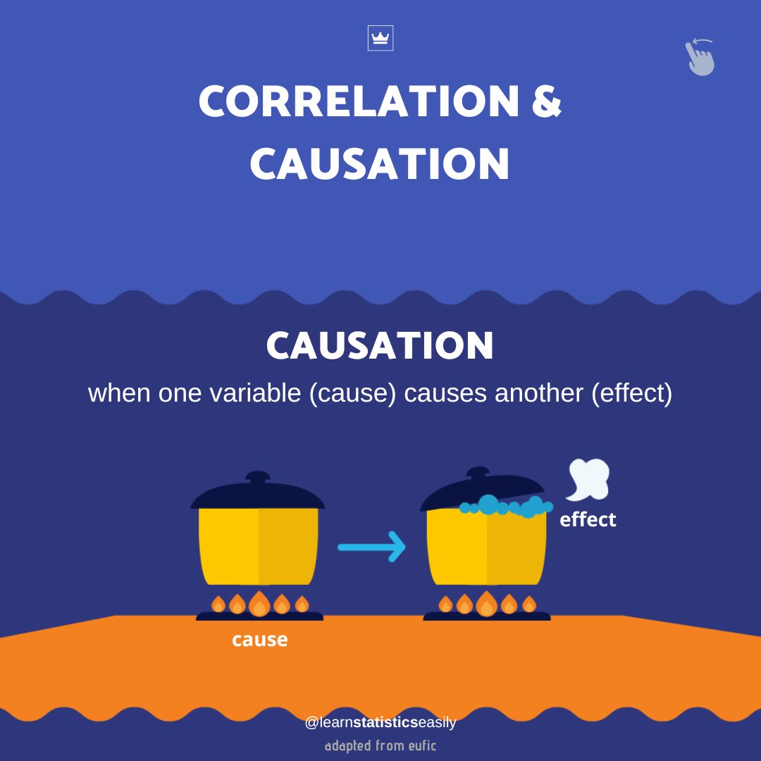
📊 In a recent study, researchers found that increasing advertising spend (independent variable) led to higher sales (dependent variable).
By analyzing the data, they established a causal relationship, helping brands make informed budget decisions.
1
5
🌟 Nominal variables may seem simple, but they hold the key to understanding complex patterns.
Embrace their diversity; every category tells a story that data can illuminate.
Let’s uncover insights together!
1
4
📊 Levene's test checks for homoscedasticity, crucial in ANOVA and regression.
It assesses if group variances are equal.
To implement, use stats libraries in Python or R.
Example: `levene(data1, data2)` in `scipy.stats`.
2
4
✨ In hypothesis testing, a p-value helps determine the significance of results.
A low p-value (typically <0.05) suggests rejecting the null hypothesis.
Type I error occurs when we incorrectly reject a true null.
Always set alpha levels wisely!
10