Acá va el código de R library(shiny) library(bslib) library(dplyr) library(readr) library(sf) library(spdep) library(leaflet) library(DT) library(stringr) library(tibble) # Exploratory spatial autocorrelation for Delitos 2025. # This does not create property-level features. It aggregates incidents to a # hex grid and checks whether counts cluster spatially. BASE_DIR <- "C:/Users/sixto/Documents/CCA_Plusvalia" OUT_DIR <- "C:/Users/sixto/Documents/Codex/2026-06-14/files-mentioned-by-the-user-library/outputs/work/delitos_2025" dir.create(OUT_DIR, recursive = TRUE, showWarnings = FALSE) DELITOS_URL <- "data.buenosaires.gob.ar/data…" DELITOS_LOCAL <- "C:/Users/sixto/Documents/Codex/2026-06-14/files-mentioned-by-the-user-library/outputs/work/spatial_raw/delitos_2025.csv" DELITOS_CACHE <- if (file.exists(DELITOS_LOCAL)) DELITOS_LOCAL else file.path(OUT_DIR, "delitos_2025_raw.csv") BARRIOS_POPULARES_URL <- "data.buenosaires.gob.ar/data…" BARRIOS_POPULARES_LOCAL <- "C:/Users/sixto/Documents/Codex/2026-06-14/files-mentioned-by-the-user-library/outputs/work/spatial_raw/barrios_populares.csv" BARRIOS_POPULARES_CACHE <- if (file.exists(BARRIOS_POPULARES_LOCAL)) { BARRIOS_POPULARES_LOCAL } else { file.path(OUT_DIR, "barrios_populares.csv") } CABA_STREETS_SHP <- file.path(BASE_DIR, "callejero/calles.shp") WORK_CRS <- 3857 norm_txt <- function(x) { x <- toupper(as.character(x)) x <- iconv(x, from = "", to = "ASCII//TRANSLIT") x[is.na(x)] <- "" trimws(x) } scaled_coord <- function(x, axis = c("lon", "lat")) { axis <- match.arg(axis) x_chr <- gsub(",", ".", as.character(x), fixed = TRUE) x_chr <- vapply(x_chr, function(v) { if (is.na(v) || !grepl("^-?\\d \\.\\d \\.", v)) return(v) sign <- if (startsWith(v, "-")) "-" else "" parts <- strsplit(sub("^-", "", v), "\\.")[[1]] paste0(sign, parts[1], ".", paste(parts[-1], collapse = "")) }, character(1)) x <- suppressWarnings(as.numeric(x_chr)) if (all(is.na(x))) return(x) limit <- if (axis == "lon") 180 else 90 for (div in c(10, 100, 1000, 10000, 100000, 1000000, 10000000)) { x <- ifelse(!is.na(x) & abs(x) > limit & abs(x / div) <= limit, x / div, x) } x } read_delitos <- function(force = FALSE) { cache_path <- DELITOS_CACHE if (force || !file.exists(cache_path)) { cache_path <- file.path(OUT_DIR, "delitos_2025_raw.csv") download.file(DELITOS_URL, cache_path, mode = "wb", quiet = TRUE) } header <- readLines(cache_path, n = 1, warn = FALSE, encoding = "UTF-8") delim <- if (str_count(header, ";") > str_count(header, ",")) ";" else "," raw <- read_delim( cache_path, delim = delim, show_col_types = FALSE, col_types = cols(.default = col_character()), locale = locale(encoding = "UTF-8") ) names(raw) <- tolower(gsub("-", "_", names(raw))) raw |> mutate( tipo_norm = norm_txt(tipo), subtipo_norm = norm_txt(subtipo), uso_arma_norm = norm_txt(uso_arma), uso_moto_norm = norm_txt(uso_moto), barrio_norm = norm_txt(barrio), lon = scaled_coord(longitud, axis = "lon"), lat = scaled_coord(latitud, axis = "lat"), cantidad_num = suppressWarnings(as.numeric(cantidad)), cantidad_num = ifelse(is.na(cantidad_num), 1, cantidad_num), grupo = case_when( str_detect(tipo_norm, "HOMICIDIO") ~ "Homicidios", str_detect(tipo_norm, "^ROBO") ~ "Robos", str_detect(tipo_norm, "^HURTO") ~ "Hurtos", TRUE ~ "Otros" ) ) |> filter( !is.na(lon), !is.na(lat), between(lon, -59, -58), between(lat, -35, -34) ) |> st_as_sf(coords = c("lon", "lat"), crs = 4326, remove = FALSE) |> st_transform(WORK_CRS) } read_barrios_populares <- function(force = FALSE) { cache_path <- BARRIOS_POPULARES_CACHE if (force || !file.exists(cache_path)) { cache_path <- file.path(OUT_DIR, "barrios_populares.csv") download.file(BARRIOS_POPULARES_URL, cache_path, mode = "wb", quiet = TRUE) } bp <- read_delim( cache_path, delim = ",", show_col_types = FALSE, col_types = cols(.default = col_character()), locale = locale(encoding = "UTF-8") ) names(bp) <- tolower(names(bp)) if (!"geometry" %in% names(bp)) return(NULL) st_as_sf(bp, wkt = "geometry", crs = 4326) |> st_make_valid() |> st_transform(WORK_CRS) } get_caba_boundary <- function() { st_read(CABA_STREETS_SHP, quiet = TRUE) |> st_transform(WORK_CRS) |> st_geometry() |> st_buffer(180) |> st_union() |> st_as_sf() |> st_make_valid() } make_hex_counts <- function(delitos, boundary, selected_groups, hex_size) { d <- delitos |> filter(.data$grupo %in% selected_groups) hex <- st_make_grid(boundary, cellsize = hex_size, square = FALSE) |> st_as_sf() |> mutate(hex_id = row_number()) |> st_filter(boundary, .predicate = st_intersects) |> st_make_valid() if (nrow(d) == 0) { hex$count <- 0 return(hex) } joined <- st_join(d, hex, join = st_within) counts <- joined |> st_drop_geometry() |> filter(!is.na(hex_id)) |> group_by(hex_id) |> summarise(count = sum(cantidad_num, na.rm = TRUE), .groups = "drop") hex |> left_join(counts, by = "hex_id") |> mutate(count = ifelse(is.na(count), 0, count)) } run_moran <- function(hex_counts) { nb <- poly2nb(hex_counts, queen = TRUE) lw <- nb2listw(nb, style = "W", zero.policy = TRUE) x <- hex_counts$count global <- moran.test(x, lw, zero.policy = TRUE) local <- localmoran(x, lw, zero.policy = TRUE) x_mean <- mean(x, na.rm = TRUE) lag_x <- lag.listw(lw, x, zero.policy = TRUE) lag_mean <- mean(lag_x, na.rm = TRUE) hex_counts |> mutate( lag_count = lag_x, local_i = local[, "Ii"], local_p = local[, "Pr(z != E(Ii))"], lisa_cluster = case_when( local_p > 0.05 ~ "No significativo", count >= x_mean & lag_count >= lag_mean ~ "High-High", count <= x_mean & lag_count <= lag_mean ~ "Low-Low", count >= x_mean & lag_count <= lag_mean ~ "High-Low", count <= x_mean & lag_count >= lag_mean ~ "Low-High", TRUE ~ "No significativo" ), moran_i = unname(global$estimate[["Moran I statistic"]]), moran_p = global$p.value, expected_i = unname(global$estimate[["Expectation"]]) ) } delitos_all <- read_delitos(force = FALSE) barrios_populares <- read_barrios_populares(force = FALSE) caba_boundary <- get_caba_boundary() ui <- page_sidebar( title = "Autocorrelacion espacial - Delitos 2025", theme = bs_theme(version = 5, bootswatch = "litera"), sidebar = sidebar( width = 330, checkboxGroupInput( "grupo", "Grupo", choices = c("Homicidios", "Robos", "Hurtos", "Otros"), selected = "Robos" ), selectInput( "hex_size", "Tamano hexagono", choices = c("500 m" = 500, "750 m" = 750, "1000 m" = 1000, "1500 m" = 1500), selected = 750 ), checkboxInput("show_bp", "Mostrar barrios populares", value = TRUE), actionButton("run", "Actualizar Moran / LISA"), hr(), tags$p( class = "small text-muted", "Moran se calcula sobre conteos agregados por hexagono. Para homicidios conviene usar hexagonos mas grandes porque son pocos eventos." ) ), navset_tab( nav_panel("LISA mapa", br(), leafletOutput("lisa_map", height = 720)), nav_panel("Moran global", br(), verbatimTextOutput("global_moran")), nav_panel("Tabla hex", br(), DTOutput("hex_table")) ) ) server <- function(input, output, session) { moran_layer <- eventReactive(input$run, { hex_counts <- make_hex_counts( delitos = delitos_all, boundary = caba_boundary, selected_groups = input$grupo, hex_size = as.numeric(input$hex_size) ) run_moran(hex_counts) }, ignoreInit = FALSE) output$lisa_map <- renderLeaflet({ x <- moran_layer() validate(need(nrow(x) > 0, "Sin hexagonos.")) x4326 <- st_transform(x, 4326) bp4326 <- if (inherits(barrios_populares, "sf")) st_transform(barrios_populares, 4326) else NULL pal_lisa <- colorFactor( palette = c( "High-High" = "#d00000", "Low-Low" = "#1d4ed8", "High-Low" = "#f97316", "Low-High" = "#22c55e", "No significativo" = "#d1d5db" ), domain = c("High-High", "Low-Low", "High-Low", "Low-High", "No significativo") ) m <- leaflet(x4326, options = leafletOptions(preferCanvas = TRUE)) |> addProviderTiles(providers$CartoDB.Positron) |> addPolygons( fillColor = ~pal_lisa(lisa_cluster), fillOpacity = ~ifelse(lisa_cluster == "No significativo", 0.18, 0.62), color = "#ffffff", weight = 0.4, popup = ~paste0( "<b>Cluster:</b> ", lisa_cluster, "<br>", "<b>Count:</b> ", count, "<br>", "<b>Lag count:</b> ", round(lag_count, 2), "<br>", "<b>Local I:</b> ", round(local_i, 4), "<br>", "<b>p:</b> ", signif(local_p, 3) ) ) |> addLegend(position = "bottomright", pal = pal_lisa, values = ~lisa_cluster, title = "LISA") if (isTRUE(input$show_bp) && inherits(bp4326, "sf") && nrow(bp4326) > 0) { m <- m |> addPolygons( data = bp4326, fillColor = "#7b2cbf", fillOpacity = 0.08, color = "#5a189a", weight = 1.1, label = ~paste0(nombre, " | ", tipo) ) } m }) output$global_moran <- renderPrint({ x <- moran_layer() cat("Grupo:", paste(input$grupo, collapse = ", "), "\n") cat("Hex size:", input$hex_size, "m\n") cat("Hexagonos:", nrow(x), "\n") cat("Eventos agregados:", sum(x$count, na.rm = TRUE), "\n\n") cat("Global Moran's I:", round(unique(x$moran_i)[1], 5), "\n") cat("Expected I:", round(unique(x$expected_i)[1], 5), "\n") cat("p-value:", signif(unique(x$moran_p)[1], 5), "\n\n") cat("Interpretacion rapida:\n") if (unique(x$moran_p)[1] <= 0.05 && unique(x$moran_i)[1] > 0) { cat("- Hay autocorrelacion espacial positiva: los conteos se agrupan.\n") } else if (unique(x$moran_p)[1] <= 0.05 && unique(x$moran_i)[1] < 0) { cat("- Hay autocorrelacion negativa: patron tipo dispersion/alternancia.\n") } else { cat("- No hay evidencia fuerte de autocorrelacion global con este grid/filtro.\n") } }) output$hex_table <- renderDT({ x <- moran_layer() |> st_drop_geometry() |> arrange(local_p) datatable( x |> select(hex_id, count, lag_count, local_i, local_p, lisa_cluster, moran_i, moran_p), rownames = FALSE, options = list(pageLength = 25, scrollX = TRUE) ) }) } shinyApp(ui, server)

[PAQUETE 📦] - [Tip de R] · shinydataviewer: Un módulo de Shiny para visualizar datos tabulares de forma interactiva. ¿Necesitás mostrar tus datos en una app de Shiny de forma prolija y con funcionalidades avanzadas, pero no querés armar todo desde cero? El paquete shinydataviewer te trae un módulo reutilizable para que tus usuarios puedan explorar tablas de datos como un pro. ✔️ data_viewer_ui() y data_viewer_server(): Integrá fácilmente un visualizador de tablas interactivas en tu app Shiny, con funcionalidades listas para usar y una estética moderna. ✔️ Tablas interactivas con reactable y bslib: Tus datos se verán geniales y serán fáciles de explorar, con búsqueda, filtrado y paginación que mejoran la experiencia de usuario. ✔️ Resumen de variables en sidebar: Tus usuarios pueden obtener un pantallazo rápido de cada columna (tipo de dato, valores únicos, distribución) sin salir de la vista principal. 💡 Tip Usá este módulo en diferentes partes de tu app para mostrar distintos datasets sin reinventar la rueda. Es ideal para dashboards que requieren exploración de datos. 🌐 ryan-w-harrison.github.io/sh… ✍️ Ryan W. Harrison #RStats #RStatsES #Rtips #DataScience

R Shiny bslib

pake shiny bslib mas

{bslib} update: #RStats #Tidyverse When `bs_theme(brand = FALSE)` we now correctly do not apply brand theming when a `_brand.yml` file is present in the project. (#1196) github.com/rstudio/bslib/blo…

{bslib} update: #RStats #Tidyverse Fixed some typos in the documentation github.com/rstudio/bslib/blo…

Asked Cursor with Claude 3.7 to give my #RStats shiny app a facelift by switching {shinydashboard} to {bslib} Spent an extra day to fix the broken bits, tweak the flows and polish the UI - but it’s still slick that I even have no idea where to start without Claude

{shinytest2} update: #RStats #Tidyverse Add support for `$click()`ing `{bslib}`'s `input_task_button()` (#389). github.com/rstudio/shinytest…

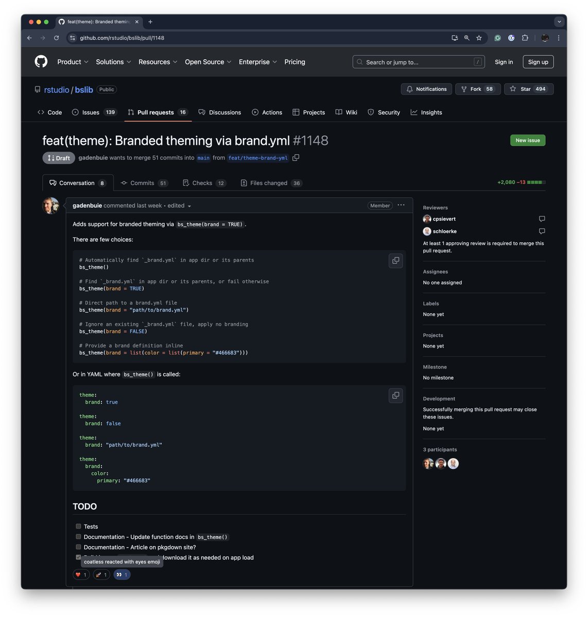
(1/2) {bslib} update: #RStats #Tidyverse bslib now supports unified theming with brand.yml. brand.yml lets you theme your Shiny apps, Quarto documents and more with a single, portable YAML file. Learn more in the new Unified theming with brand.yml article. (#1148)

What's this I spy? #brandyml support appears to be on the horizon in {bslib} for #rstats #shiny. Could this be an early Christmas gift? 🎁 github.com/rstudio/bslib/pul…

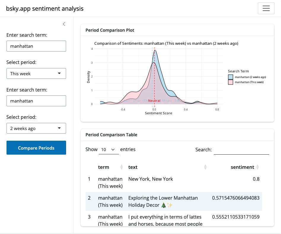
I just updated my sentiment analysis app. Using bslib makes it much prettier! The sentiment for "Manhattan" has shifted negatively compared to two weeks ago (we all know why). Try the app here: editor.ploomber.io/app/d2a65… #rstats

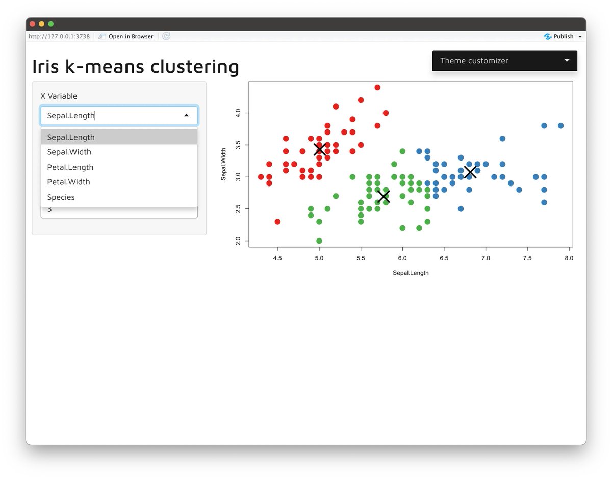
1. Janitor: Simplifying Data Cleaning 2. Skimr: Quick Data Summarization 3. bslib: Next-Gen UI for Shiny Apps 4. box: Modularize Your R Scripts 5. data.table & tidytable: High-Performance Data Manipulation

📢 Missed out on the #RMedicine 2024 talk "Next Generation Shiny Apps with {bslib}"? 🌟 No worries, the recording is now on YouTube! 🎥 Learn how {bslib} can elevate your Shiny app development. Watch here: youtube.com/watch?v=vzXTFbnK… #RStats #Shiny #DataScience #HealthTech

1. Janitor: Simplifying Data Cleaning 2. Skimr: Quick Data Summarization 3. bslib: Next-Gen UI for Shiny Apps 4. box: Modularize Your R Scripts 5. data.table & tidytable: High-Performance Data Manipulation

1. Janitor: Simplifying Data Cleaning 2. Skimr: Quick Data Summarization 3. bslib: Next-Gen UI for Shiny Apps 4. box: Modularize Your R Scripts 5. data.table & tidytable: High-Performance Data Manipulation

Learn more about bslib here: rstudio.github.io/bslib/

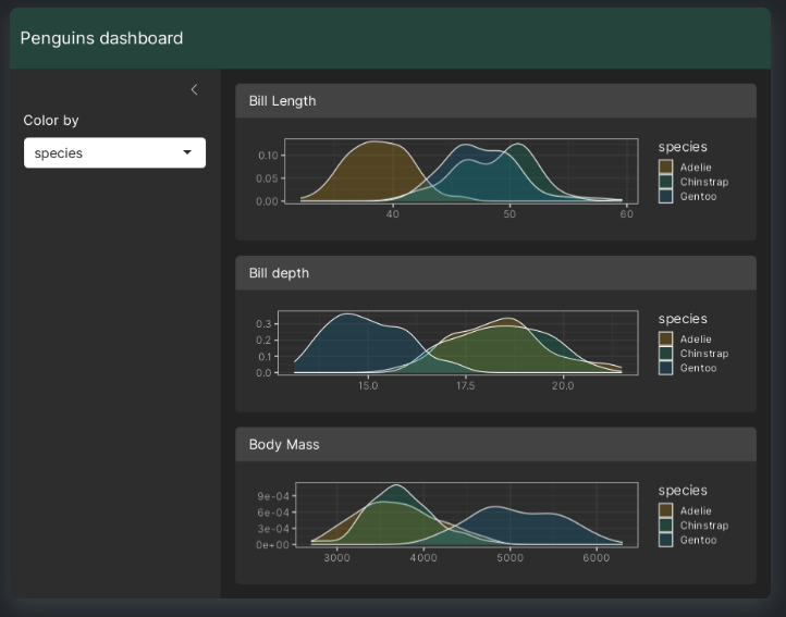
With bslib, you can make powerful applications with fewer lines of code because bslib supports: - Cards - Layouts - Widgets

bslib is an R package that provides a modern UI toolkit for Shiny and R Markdown based on Bootstrap.

"You can't deploy in R." BS... You CAN with bslib.

Yes I have one on bslib coming tomorrow.