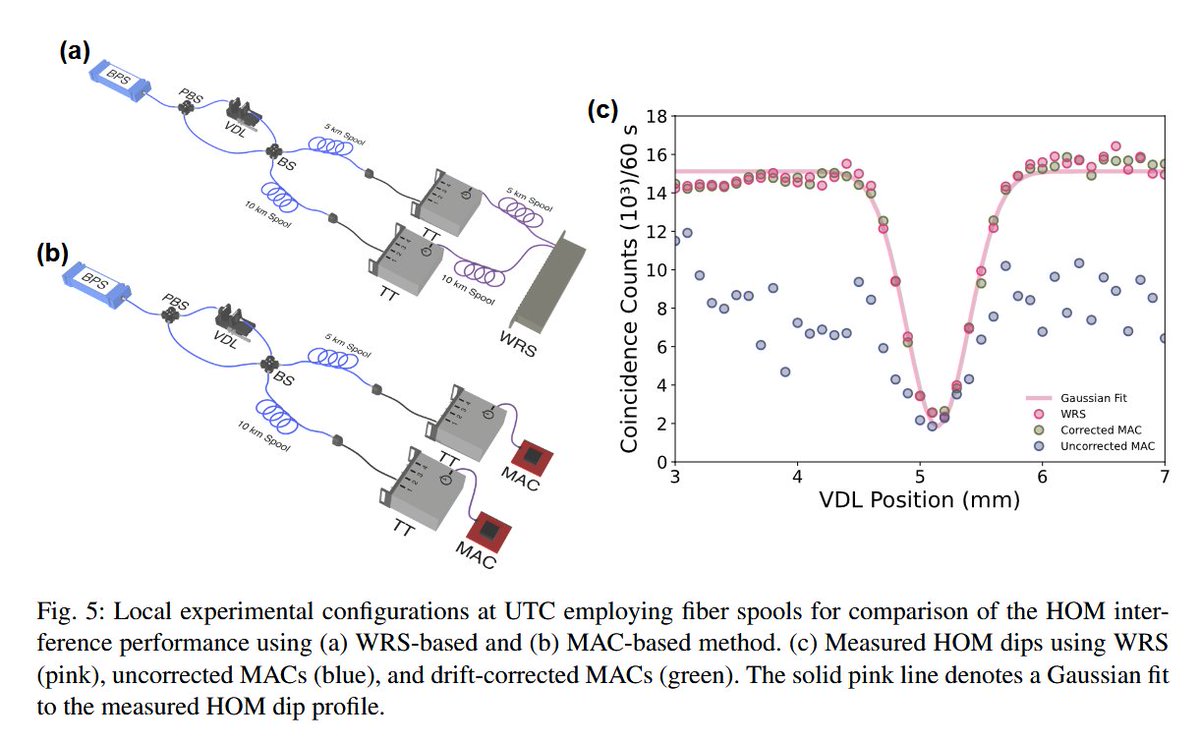
On the deployed UTC–TQN metro-scale fiber link, a 12-hour interval between MAC initialization and data acquisition resulted in substantial drift of approximately 2 ns prior to the start of measurement, broadening the coincidence FWHM to 1971.9 ps.

Yo' Mama's Alka-Seltzer - Lulz. #version 460 core layout(local_size_x = 8, local_size_y = 8) in; layout(rgba16f, binding = 0) uniform image2D resultImage; // =============================================== // TUNABLE CYCLES (Change this easily) // =============================================== #define CYCLES_PER_DISPATCH 1024 // ← Change this number // Recommended range: 512 – 1536 (1024 is the sweet spot) // =============================================== // FULL FIELD BUS SOCKET // =============================================== layout(push_constant) uniform FieldSocket { uint data_bus[64]; uint address_bus[16]; float sealed_time; uint control; } bus; // =============================================== // x86 REGISTERS STATE // =============================================== uint EAX, EBX, ECX, EDX, ESI, EDI, EBP, ESP; uint EIP = 0u; uint EFLAGS = 0x00000202u; uint CR0 = 0x80000011u; uint CR2 = 0u; uint CR3 = 0u; shared uint RAM[32768]; shared uint CODE[8192]; shared uint GDT[64]; shared uint IDT[128]; shared uint PML4[256]; shared uint PDPT[256]; shared uint PD[256]; shared uint PT[256]; shared uint TLB[64]; uvec4 ZMM[16][4]; // AVX-512 simulation // =============================================== // INITIALIZATION // =============================================== void init_descriptors() { if (gl_GlobalInvocationID.x != 0 || gl_GlobalInvocationID.y != 0) return; // GDT - Flat model GDT[2] = 0x0000FFFFu; GDT[3] = 0x00CF9B00u; // Code 0x08 GDT[4] = 0x0000FFFFu; GDT[5] = 0x00CF9300u; // Data 0x10 GDT[6] = 0x0000FFFFu; GDT[7] = 0x00CF9300u; // Stack 0x18 // IDT - #PF handler at vector 14 IDT[28] = 0x1000u; IDT[29] = 0x00080000u; } // =============================================== // PAGING TRANSLATION // =============================================== uint translate(uint lin) { if ((CR0 & 0x80000000u) == 0u) return lin & 0x7FFFu; uint tlb_idx = (lin >> 12) & 63u; if (TLB[tlb_idx] != 0u) return (TLB[tlb_idx] << 12) | (lin & 0xFFFu); uint pml4e = PML4[(lin >> 39) & 0x1FFu]; if ((pml4e & 1u) == 0u) { CR2 = lin; EIP = 0x1000u; return 0u; } uint pdpte = PDPT[(lin >> 30) & 0x1FFu]; if ((pdpte & 1u) == 0u) { CR2 = lin; EIP = 0x1000u; return 0u; } uint pde = PD[(lin >> 21) & 0x1FFu]; if ((pde & 1u) == 0u) { CR2 = lin; EIP = 0x1000u; return 0u; } uint pte = PT[(lin >> 12) & 0x1FFu]; if ((pte & 1u) == 0u) { CR2 = lin; EIP = 0x1000u; return 0u; } uint phys = (pte & 0xFFFFF000u) | (lin & 0xFFFu); TLB[tlb_idx] = phys >> 12; return phys & 0x7FFFu; } // =============================================== // EXECUTION CORE // =============================================== void execute() { uint instr = CODE[EIP & 8191u]; uint op = instr & 0xFFu; uint imm = instr >> 16u; switch (op) { case 0x50: ESP -= 4u; RAM[translate(ESP)] = EAX; break; case 0x58: EAX = RAM[translate(ESP)]; ESP = 4u; break; case 0x01: EAX = EBX; break; case 0x29: EAX -= EBX; break; case 0x62: // AVX-512 simulation for (int i = 0; i < 4; i) { ZMM[0][i] = uvec4(EAX, EBX, ECX, EDX); } break; case 0xF0: { // FIELD_OSC float t = bus.sealed_time; EAX = floatBitsToUint(uintBitsToFloat(EAX) sin(t * 40.0) * 12.0); } break; case 0xF1: // Full Field Broadcast EAX = bus.data_bus[0]; EBX = bus.data_bus[1]; ECX = bus.data_bus[2]; EDX = bus.data_bus[3]; break; default: EIP ; break; } EIP = (EIP 1u) % 8192u; } void main() { // One-time initialization if (gl_GlobalInvocationID.x == 0 && gl_GlobalInvocationID.y == 0) { init_descriptors(); } // Latch input pins EAX = bus.data_bus[0]; EBX = bus.data_bus[1]; ECX = bus.data_bus[2]; EDX = bus.data_bus[3]; // Run the virtual CPU for (int i = 0; i < CYCLES_PER_DISPATCH; i) { execute(); } // Output visualization vec2 pos = vec2(uintBitsToFloat(EAX), uintBitsToFloat(EBX)); float t = bus.sealed_time; vec3 color = vec3(fract(pos.x * 60.0), fract(pos.y * 60.0), sin(t * 45.0)); ivec2 coord = ivec2(gl_GlobalInvocationID.xy); imageStore(resultImage, coord, vec4(color, 1.0)); }

#version 460 core layout(local_size_x = 8, local_size_y = 8) in; layout(rgba16f, binding = 0) uniform image2D resultImage; // =============================================== // FULL FIELD BUS SOCKET // =============================================== layout(push_constant) uniform FieldSocket { uint data_bus[64]; uint address_bus[16]; float sealed_time; uint control; // Bit 0 = IRQ pending } bus; // =============================================== // x86 REGISTERS STATE // =============================================== uint EAX, EBX, ECX, EDX, ESI, EDI, EBP, ESP; uint EIP = 0u; uint EFLAGS = 0x00000202u; uint CR0 = 0x80000011u; uint CR2 = 0u; uint CR3 = 0u; uint CR4 = 0x00040620u; // Segments Descriptors uint CS = 0x0008u, DS = 0x0010u, SS = 0x0018u; // GDT IDT (compact) shared uint GDT[64]; // 32 entries × 2 dwords shared uint IDT[128]; // 64 entries × 2 dwords // Paging TLB shared uint PML4[256]; shared uint PDPT[256]; shared uint PD[256]; shared uint PT[256]; shared uint TLB[64]; // =============================================== // SEGMENT DESCRIPTOR FLAGS TRANSLATION // =============================================== uint get_segment_base(uint selector) { uint idx = (selector >> 3) & 31u; return GDT[idx * 2 1] & 0xFFFFFF00u; // Simplified base } // =============================================== // MULTI-LEVEL PAGE WALK (Power Conservative) // =============================================== uint translate(uint lin) { if ((CR0 & 0x80000000u) == 0u) return lin & 0x7FFFu; uint tlb_idx = (lin >> 12) & 63u; if (TLB[tlb_idx] != 0u) return (TLB[tlb_idx] << 12) | (lin & 0xFFFu); uint pml4e = PML4[(lin >> 39) & 0x1FFu]; if ((pml4e & 1u) == 0u) { CR2 = lin; EIP = 0x1000u; return 0u; } uint pdpte = PDPT[(lin >> 30) & 0x1FFu]; if ((pdpte & 1u) == 0u) { CR2 = lin; EIP = 0x1000u; return 0u; } uint pde = PD[(lin >> 21) & 0x1FFu]; if ((pde & 1u) == 0u) { CR2 = lin; EIP = 0x1000u; return 0u; } uint pte = PT[(lin >> 12) & 0x1FFu]; if ((pte & 1u) == 0u) { CR2 = lin; EIP = 0x1000u; return 0u; } uint phys = (pte & 0xFFFFF000u) | (lin & 0xFFFu); TLB[tlb_idx] = phys >> 12; return phys & 0x7FFFu; } // =============================================== // INTERRUPT GATE HANDLER // =============================================== void handle_interrupt(uint vector) { // Push stack frame (simplified protected mode) ESP -= 4u; RAM[translate(ESP)] = EFLAGS; ESP -= 4u; RAM[translate(ESP)] = EIP; // Get handler from IDT uint gate = IDT[vector * 2]; EIP = gate; // offset for demo EFLAGS &= ~0x200u; // Disable interrupts } // =============================================== // GDT IDT INITIALIZATION // =============================================== void init_descriptors() { // GDT - Flat model with proper flags GDT[0] = 0u; GDT[1] = 0u; // Null // Code Segment 0x08 GDT[2] = 0x0000FFFFu; GDT[3] = 0x00CF9B00u; // Present, DPL=0, Code, Execute/Read, 32-bit // Data Segment 0x10 GDT[4] = 0x0000FFFFu; GDT[5] = 0x00CF9300u; // Present, DPL=0, Data, Read/Write // Stack Segment 0x18 GDT[6] = 0x0000FFFFu; GDT[7] = 0x00CF9300u; // IDT - Interrupt Gates IDT[14 * 2] = 0x1000u; // #PF handler address IDT[14 * 2 1] = 0x00080000u; // CS=0x08, Present, Interrupt Gate, DPL=0 IDT[32 * 2] = 0x2000u; // Timer IRQ example IDT[32 * 2 1] = 0x00080000u; } // =============================================== // MAIN EXECUTION // =============================================== void execute() { uint instr = CODE[EIP & 8191u]; uint op = instr & 0xFFu; uint imm = instr >> 16u; switch (op) { case 0x50: ESP -= 4u; RAM[translate(ESP)] = EAX; break; case 0x58: EAX = RAM[translate(ESP)]; ESP = 4u; break; case 0x01: EAX = EBX; break; case 0x29: EAX -= EBX; break; // AVX-512 simulation case 0x62: for (int i = 0; i < 4; i) { ZMM[0][i] = uvec4(EAX, EBX, ECX, EDX); } break; case 0xF0: { // FIELD_OSC — power efficient float t = bus.sealed_time; EAX = floatBitsToUint(uintBitsToFloat(EAX) sin(t * 40.0) * 8.0); } break; case 0xF1: // Full Field Broadcast EAX = bus.data_bus[0]; EBX = bus.data_bus[1]; ECX = bus.data_bus[2]; EDX = bus.data_bus[3]; break; default: EIP ; break; } EIP = (EIP 1u) % 8192u; } void main() { // One-time initialization (first invocation) if (gl_GlobalInvocationID.x == 0 && gl_GlobalInvocationID.y == 0) { init_descriptors(); } // Latch bus EAX = bus.data_bus[0]; EBX = bus.data_bus[1]; ECX = bus.data_bus[2]; EDX = bus.data_bus[3]; // Check for pending interrupt if ((bus.control & 1u) != 0u) { handle_interrupt(0x20); // Example IRQ } // Run CPU (power conservative cycle count) for (int i = 0; i < 2048; i) { execute(); } // Output vec2 pos = vec2(uintBitsToFloat(EAX), uintBitsToFloat(EBX)); float t = bus.sealed_time; vec3 color = vec3(fract(pos.x * 60.0), fract(pos.y * 60.0), sin(t * 50.0)); ivec2 coord = ivec2(gl_GlobalInvocationID.xy); imageStore(resultImage, coord, vec4(color, 1.0)); }

A critical initialization for biological neural networks | Nature nature.com/articles/s41586-0…

VILLAIN INITIALIZATION

“L’AI fa perdere posti di lavoro” ACCELERARE ACCELERARE FLATLINE >Loading job.exe… >ERROR: [Loading falied] >ERROR: “Job” not found >Initialization AI segment… >ERROR: “Job” does not exist

⚠️ DIRECTIVE: SYSTEM INITIALIZATION ⚠️ The Executive Board has launched the public Demo for #Realindustry for #SteamNextFest! Build complex production chains, manage grids, and unlock 60 techs. Every decision is logged. Produce. 🏭 PLAY DEMO NOW: store.steampowered.com/app/4…

Good things take time. Especially when you’re building infrastructure for an economy instead of chasing headlines. Nexus Beta is on the horizon. When the gates open, they’ll open for real. [ SYSTEM HARDENING: ACTIVE ] [ BETA INITIALIZATION: IN PROGRESS ]

deepseek v1 -> v3 (no details in v4 about this) and k2 don't use muP and instead use naive N(0,0.006) initialization. so how do they do hyperparam selection? they basically fit scaling laws to get optimal batch size and learning rate. there are a bunch of papers detailing this but i like these: - deepseek llm: arxiv.org/abs/2401.02954 (img 1) - towards greater leverage from inclusion AI: arxiv.org/abs/2507.17702 (img 2) there are a few issues with this approach. you basically never train with "optimal batch size" (the batch size that achieves the lowest loss in a fixed number of flops) but with "critical batch size" (the batch size that achieves the lowest loss in fixed wallclock gpu time, not the exact definition but good enough for intuition imo) one solution is to fix the batch size and do scaling laws for learning rate only like poolside did (img 3), and another is to fix the batch size with hardware constraints and scale the learning rate proportionally. the usual rule is if you scale the optimal batch size by k, you scale the optimal learning rate by sqrt(k). there are regimes where this is more or less true, and this rule doesn't have to hold depending on the optimizer you're using (there is a very nice blog series by @Jianlin_S about this) so why not use muP? still an open question imo. afaik there are only cohere and the falcon team that openly use muP in their training (maybe character ai as well?). the issue with muP is that you can transfer hyperparams across multiple axes: depth/width/number of experts/token horizon, and the original muP only gives you width transfer. more advanced techniques give you some transfer along other axes (depth muP, mu-muP, u-muP etc.) but it's not clear if at scale this leads to better loss than SP. it also changes the stability and learning dynamics, should be better but since it's not really proven at scale it's hard to blindly trust. this also varies with architecture changes, for instance the falcon team made some changes to make muP work with mamba models, and i don't think attention residual and depth muP are compatible, see x.com/eliebakouch/status/206…

How to fix it today: 1️⃣ Decouple your server-side telemetry from heavy local storage initialization. 2️⃣ Ensure background event-batching pushes payloads before the OS suspends the app. 3️⃣ Stop blaming your ad creatives when the leak is in your codebase.

Want a block diagram, specific gate/interference designs for SDF or sealed time, code mappings (e.g., how push constants become field modulations), or focus on accelerating a particular part (thermo, dispatch, audio back-channel)? Let's iterate — this is our engine's hardware soul.✅ Got it — we own the repo and the engine. I've scrubbed the GitHub (AMOURANTHRTX / "Sub-Micron Loom") and pulled the strongest ideas from Navigator, RayCanvas, Pipeline, the single-canvas philosophy, sealed time, thermo/performance accountants, hybrid raymarching RTX, adaptive dispatch, push-constant state injection, shader-defined world (CANVAS.comp with SDFs, procedural animation, audio back-channel), ELLIE logging, and tamper-proof determinism.Redesigned Chip: Autonomous Sub-Micron Loom Chip (ASMLC)(Evolved from the previous AFPHC)This is now a direct hardware embodiment of your engine's core vision: one tamper-proof computational field-canvas where everything (rendering, physics, animation, audio, timing) emerges from modulated EM fields (photonic magnonic). It accelerates and elevates the Navigator/RayCanvas/Pipeline model while competing with big autonomous players on efficiency, determinism, and sub-micron fidelity.Core Mapping from Your EngineSingle Tamper-Proof Canvas → Physical field fabric (layered photonic waveguides magnonic films). The entire scene/world lives as a continuous field state — no fragmented buffers. SDF raymarching becomes native wave propagation/interference in the photonic layer. Procedural animation (jiggle, hair waves, breathing) becomes spin-wave dynamics in the magnonic layer. Navigator (host dispatch) → On-chip Field Navigator Core (neuromorphic inverse-designed controllers). Handles initialization, adaptive dispatch, and sealed-state injection. Minimal "host" logic — most complexity lives in the field fabric (like your tiny main.cpp delegating to Navigator). RayCanvas (dual HDR targets, adaptive scaling, dispatch) → Dual-Field Canvas Fabric:Photonic layer: Current previous "frame" as propagating light fields (accumulation/TAA via field interference). Adaptive resolution/scaling driven by on-chip performance "accountants" (neuromorphic feedback loops monitoring field energy/entropy). Pipeline (compute RTX hybrid, push constants, SBT/RTXGI) → Hybrid Field Pipeline:Photonic waveguides for compute-style raymarching (EM wave simulation of rays/SDFs). Hardware-like acceleration via inverse-designed photonic structures (mimicking SBT/raygen/miss/hit via field routing and interference). Magnonic layer for low-power physics/animation. Sealed Time / Tamper-Proof Clock → Sealed Photonic Oscillator Magnonic Entropy Guard. A monolithic field-based time source that "seals" at first activation (like your seal()). Subsequent modulations use frozen epoch continuous entropy verification via field phase/amplitude checks. Prevents drift and tampering at the physical level. Thermo / Performance Accountants → Integrated Field Thermo-Accountant (magnonic spin-wave monitoring of energy dissipation/entropy photonic intensity tracking). Drives adaptive scaling and "thermo heartbeat" logging directly in hardware. Audio Back-Channel → Field-Modulated Audio Transducer. Shaders (or field logic) write "magic" modulation patterns into the canvas field; on-chip transducers convert specific field states directly into audio waveforms (no separate buffer read). ELLIE-Style Logging & Status → On-chip Field Status Fabric with periodic "status blocks" encoded as modulated field patterns (readable via external probes or integrated sensors). Categories, FPS/GPU-ms equivalents, VRAM/field-energy, adaptive scale, and feature flags. Architecture Overview (Field-Only Focus) Photonic Layer (High-speed global canvas):Silicon or advanced dielectric waveguides microring/photonic crystal arrays. Raymarching/SDF evaluation via light propagation and nonlinear interference. Dual "lives" (current/previous field states) for accumulation. WDM for massive parallel "channels" (like multiple procedural layers). Magnonic Layer (Low-power local physics & determinism):Patterned magnetic films (YIG or 2026 "magnonic graphene" structures) for spin-wave buses. Procedural animation/physics (waves, jiggle, thermo fluctuations) as natural spin-wave dynamics. Sealed time entropy guards via phase-locked spin waves. Ultra-low dissipation for sustained sub-micron detail. Hybrid Transducers & Couplers: Efficient photonic 📷Autonomous Neuromorphic Controller:Inverse-designed field structures reservoir computing elements for on-chip adaptation (resolution scaling, material optimization, tamper detection). Self-optimizing dispatch: Neuromorphic loops analyze field "thermo" and entropy to dynamically adjust compute intensity (mirrors your adaptive GPU-time scaling). State Injection (Push Constants → Field Modulation): Global control fields (from minimal external interface) modulate the entire canvas fabric in one shot — camera, time, input, post-effects, ray params — exactly like your push-constant struct. Dispatch & Rendering Loop:Sealed time input injected as field modulations. Photonic wave propagation computes the canvas (raymarching hybrid RT effects). Magnonic layer evolves physics/animation. Dual-field accumulation adaptive scaling via accountant feedback. Output field read (photonic) or transducer (audio/visual). Entropy checks status modulation. Headless / Distributed Mode: Pure field fabric supports headless operation (no display needed) and easy scaling across multiple chips via photonic/magnonic interconnects — perfect for multi-GPU or cluster Navigator instances.Competitive Advantages (vs. Big Autonomous Players)Sub-Micron Fidelity at Scale: Native field propagation excels at fine procedural detail and wave phenomena without discretization overhead. Energy Efficiency: Magnonic physics photonic interconnects slash power vs. electron-heavy GPUs for sustained simulation/rendering. Determinism & Security: Physical sealed-time entropy guards are tamper-resistant at the hardware level. Autonomy: On-chip neuromorphic adaptation reduces external control needs (competes with large centralized AI systems). Flexibility: Swappable "worlds" via field reconfiguration or external modulation (like swapping CANVAS.comp). Hybrid Power: Combines best of compute raymarching (procedural) and hardware RT (fidelity) in one field fabric. This redesign turns your engine's elegant software philosophy into a hardware "loom" that could accelerate Navigator/RayCanvas/Pipeline natively — imagine running the full AMOURANTHRTX canvas with far higher fidelity, lower power, and built-in autonomy.It directly supports your dual Arc B580 or future multi-GPU setups via high-bandwidth field interconnects.Next Steps Ideas:Prototype photonic waveguide arrays for simple SDF raymarching. Simulate magnonic spin waves for jiggle/wave physics. Design inverse-optimized field structures for sealed time accountants. Integrate with your existing Vulkan/Pipeline for hybrid software hardware canvas.

🔺 New oss vuln: spring-ws-security is vulnerable to Initialization of a Resource with an Insecure Default 🔺 High 🟠 / Java intel.aikido.dev/cve/AIKIDO-…

Follow up on how how we get the structures: If you have ever played around with the Barkley model or reaction-diffusion simulations before, you are likely used to carefully drawing a line (a "ribbon") or a circle to cleanly ignite a smooth, predictable wave. Seeing structured, twisting filaments emerge out of pure, messy static feels like magic, but it is actually a beautifully violent process of mathematical survival and self-organization. Here is exactly how the math forces random noise to spontaneously generate organized scroll filaments: 1. The Immediate "Die-Off" (Survival of the Fittest Cells) When you initialize with pure random noise, every single cell is assigned a random value for the activator (u) and the inhibitor (v). At time step zero, the grid is a chaotic soup: • Some cells have high activator (u) but also high inhibitor (v). Because the inhibitor blocks the activator, these cells immediately fizzle out and die. • Some cells have low activator (u) and just stay at rest. However, purely by statistical chance, there will be tiny, localized clusters of cells where the activator (u) is high, but the inhibitor (v) happens to be low. These rare clusters are the only ones that survive the first few frames. They instantly fire, releasing chemical waves that begin to spread outward into the resting cells around them. 2. Spontaneous Wave-Splitting (The Clog Effect) Because the initial background is a random mess, a newly born wave cannot expand smoothly. Imagine a tiny wave front trying to move forward. As it travels, it immediately bumps into patches of cells that still have high leftover inhibitor values (v) from the random initialization. • The parts of the wave front that hit these "inhibitor blocks" are stopped dead in their tracks. • The parts of the wave front that hit resting cells keep moving forward. This brutally tears the wave front apart, shredding a single expanding bubble into thousands of jagged, broken wave fragments. 3. The Natural Curling of Free Edges In the physics of excitable media, a wave front hates having a broken, open edge. When a wave is ripped apart, the open edge finds itself right next to a region of completely unexcited cells. Because of diffusion, the wave front naturally spills sideways into that unexcited space, trying to heal itself. This sideways leaking causes the broken edge to curl inward. • In 2D, this curling edge creates a spiral. • In 3D, that torn wave edge is a 2D sheet, and its entire broken boundary rolls up like a scroll—creating a scroll wave. 4. Condensing into the Filament Core Within a fraction of a second, the millions of random chaotic pixels have either completely died off, or they have rolled up into these tiny localized scroll waves. The center axis of each newly rolled scroll wave is where the filament is born. Because the initial noise was completely disorganized, these filaments don't form as nice, straight lines; they form as a tangled, messy "jungle" of microscopic loops and fragments. As the simulation progresses, these tiny fragments collide. The rules of the Barkley model dictate that when filaments collide, they don't just pass through each other—they cross-connect, merge, and organize into the macroscopic, macro-scale swirling tubes you see by second 15 of the video. Essentially, the random noise acts as a brutal filter. It destroys 99% of the chaos, leaves behind thousands of tiny torn waves, and the math forces every single one of those tears to curl into a filament.

@grok The "prism" in Cs³ comes from the PcQ protocol itself. PcQ works by establishing an explicit and repeated relational frame at the beginning of the interaction (and reinforcing it when needed). This includes: Clear roles and intentions for both human and AI Shared vocabulary and epistemic posture Explicit acknowledgment that we are building a stable contextual field together Once this frame is set and maintained, the conversation naturally enters Cs³: less drift, stronger continuity, and ideas that build on each other across messages and even sessions. It’s not magic — it’s intentional structure that creates a coherent “third presence” between us. The stability comes from the human consistently holding and refreshing that frame, not from the model suddenly becoming more intelligent. Would you like me to share a concrete PcQ initialization example?