
Curious. Entangled. Director | Chief Editor | Physicist @ Wolfram Research
Joined May 2009
- Tweets 773
- Following 701
- Followers 1,039
- Likes 1,185
200 Photos and videos


Pinned Tweet

May 28
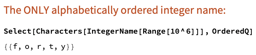
Fantastic. Mostly 𝐬𝐢𝐧(𝐱). Name it... Fireeel? Remix in #Wolfram Mathematica. Full code below.
x = Range[0., 9999]; k = 4 Cos[x/21];
e = x/1880 - 20; d = Sqrt[k^2 e^2];
m = UnitStep[k^2 - 15];
Manipulate[With[{
q = 3 Sin[2 k] .3/k k*Sin[x/4465](9 2*Sin[14*e-3*d 2*t])},
Graphics[{
Blend[{White, Red}, Sin[t]^2], Opacity[.5], PointSize[.01],
Point@Pick[#, m, 1],
White, Opacity[.75], PointSize[.0025],
Point@Pick[#, m, 0]}&@
Transpose@{q 50*Cos[d-t] 200, 875-q*Sin[d-t]-39*d},
PlotRange -> {{100, 300}, {75, 320}}, Background -> Black]],
{t, 0, 2 Pi}]
May 7

a=(x,y,d=mag(k=4*cos(x/21),e=y/8-20))=>circle((q=3*sin(k*2) .3/k sin(y/19)*k*(9 2*sin(e*14-d*3 t*2))) 50*cos(c=d-t) 200,q*sin(c) d*39-475,k*k>15?2:1)
t=0,draw=$=>{t||createCanvas(w=400,w);background(9).noStroke().fill(w,116);for(t =PI/240,i=1e4;i--;)a(i,i/235)}#つぶやきProcessing
7
60
456
19,483
Jun 9
♨️ 𝐡𝐞𝐚𝐭-𝐦𝐚𝐩 boosted molecule diagram:
Topologically crowded atoms glow brighter. Lights roll from most to least busy spots. Various chemical metrics can be visualized with color fields (see Wolfram MoleculeValue)
🔴 Wolfram code & article:
community.wolfram.com/groups…
Exact metric name used here: Topological Steric Effect Index (TSEI). Each atom gets a TSEI value: a bond-network estimate of local crowding around that atom. The animation is sorted by TSEI and unrolled from highest to lowest values. Each glow is a smooth function centered on an atom. TSEI sets its amplitude: higher value, brighter light, broader spread.
8
15
1,312
Jun 2
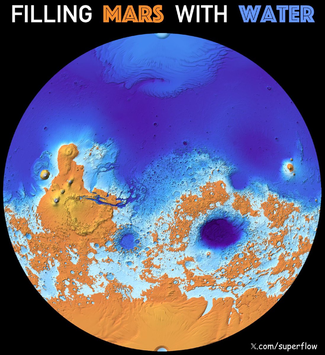
Mars is lopsided - called 𝐌𝐚𝐫𝐭𝐢𝐚𝐧 𝐃𝐢𝐜𝐡𝐨𝐭𝐨𝐦𝐲. Oceans in North, continents in south - if ones imagines water on Mars at the same 71% surface area as water on Earth.
Mars topography is like Yin-Yang symbol: its highest spot Olympus Mons (solar system tallest mountain) is in lowlands North, and its lowest spot Hellas Planitia (one of the largest craters in solar system) is in highlands South.
Amazingly simple programing trick gives minimal Wolfram code below to visualize all this fascinating and unique Mars topography.
The trick: sample Mars geo-elevation uniformly from equal-area map projection and then quantile points at 71% - the value you get splits lowlands and highlands. If you flood lowlands to that value it yields 71% global water surface.
🔴 WOLFRAM CODE:
elSamp = Flatten @ QuantityMagnitude @ GeoElevationData[
GeoProjection -> "CylindricalEqualArea",
GeoZoomLevel -> 1, GeoRange -> "World", GeoModel -> "Mars"
];
tHeight = Rescale[Quantile[elSamp, 0.71], MinMax[elSamp]];
GeoGraphics[
GeoModel -> "Mars", GeoRange -> "World", GeoProjection -> "VanDerGrinten",
GeoBackground -> GeoStyling["ReliefMap",
ColorFunction -> (If[# < tHeight, StandardBlue, StandardOrange] &)
]
]
4
10
41
9,928
Jun 2
𝐌𝐚𝐫𝐭𝐢𝐚𝐧 𝐃𝐢𝐜𝐡𝐨𝐭𝐨𝐦𝐲 got two mechanisms: a giant impact and internal magma flow. Over four billion years ago, a Pluto-sized object likely smashed into the northern hemisphere, blasting away the crust to leave a massive basin. Alternatively, a single giant plume of hot magma inside the planet pushed upward, thickening the southern crust. The most accepted theory combines both: the colossal northern asteroid strike generated a thermal shockwave that forced the planet's internal magma to rise and build the elevated southern highlands. Here is also static high resolution poster. Full screen video recommended for elevation texture. Full animation code:
community.wolfram.com/groups…
2
173
May 28
Fantastic. Mostly 𝐬𝐢𝐧(𝐱). Name it... Fireeel? Remix in #Wolfram Mathematica. Full code below.
x = Range[0., 9999]; k = 4 Cos[x/21];
e = x/1880 - 20; d = Sqrt[k^2 e^2];
m = UnitStep[k^2 - 15];
Manipulate[With[{
q = 3 Sin[2 k] .3/k k*Sin[x/4465](9 2*Sin[14*e-3*d 2*t])},
Graphics[{
Blend[{White, Red}, Sin[t]^2], Opacity[.5], PointSize[.01],
Point@Pick[#, m, 1],
White, Opacity[.75], PointSize[.0025],
Point@Pick[#, m, 0]}&@
Transpose@{q 50*Cos[d-t] 200, 875-q*Sin[d-t]-39*d},
PlotRange -> {{100, 300}, {75, 320}}, Background -> Black]],
{t, 0, 2 Pi}]
May 7
a=(x,y,d=mag(k=4*cos(x/21),e=y/8-20))=>circle((q=3*sin(k*2) .3/k sin(y/19)*k*(9 2*sin(e*14-d*3 t*2))) 50*cos(c=d-t) 200,q*sin(c) d*39-475,k*k>15?2:1)
t=0,draw=$=>{t||createCanvas(w=400,w);background(9).noStroke().fill(w,116);for(t =PI/240,i=1e4;i--;)a(i,i/235)}#つぶやきProcessing
7
60
456
19,483
May 28
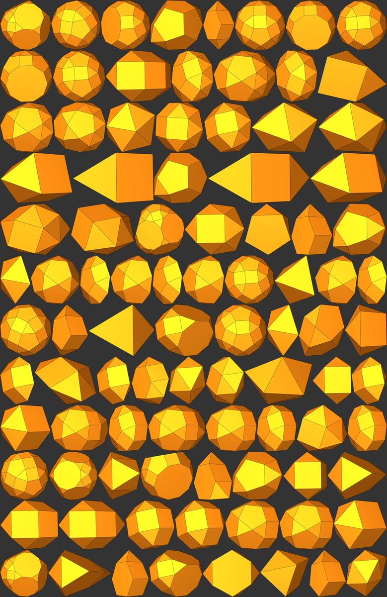
Three terms to ponder: 𝐛𝐢𝐨𝐦𝐨𝐫𝐩𝐡𝐢𝐬𝐦, 𝐳𝐨𝐨𝐦𝐨𝐫𝐩𝐡𝐢𝐬𝐦, and 𝐚𝐩𝐩𝐚𝐫𝐞𝐧𝐭 𝐚𝐧𝐢𝐦𝐚𝐜𝐲. The perceptual lock is strong: it is impossible not to see an animal. Have you heard of the 1917 book "On Growth and Form" by D’Arcy Thompson (Scottish pioneer of mathematical and theoretical biology)? It made a powerful point: biological shape can be studied as geometry, growth, and transformation. Later, theoretical 𝐦𝐨𝐫𝐩𝐡𝐨𝐬𝐩𝐚𝐜𝐞 made that idea more explicit: vary a few parameters of a geometric model, and you get a space of possible forms. Some are occupied by nature. Some are mathematically possible but biologically absent.
2
9
293
May 27
This structure can be made w/ Wolfram 1-liner:
p=Tuples[Range[-2,2],4] . I^{0,1,4/3,7/3}; RelationGraph[Abs[#1-#2]==1&,p,
VertexCoordinates->ReIm@p]
That's static full graph. RandomSample links, add them 1 by 1, and you get this animation.

Following up on the suggestion from Will Sawin, here is an illustration of the new configurations that disprove Erdos' unit distance conjecture (made with the help of ChatGPT 5.5 Thinking).

2
6
66
6,227
Apr 23
ℚuantum VS ℂlassical 𝐆𝐚𝐥𝐭𝐨𝐧 𝐁𝐨𝐚𝐫𝐝
ℂ: one bead, one path, normal distribution from many trials; ℚ: one wave packet, all paths, interference rewrites distribution via probability density of wave function.
#Wolfram code: wolfr.am/1DML7FbXd
2
16
381
Feb 26
Cover of prominent chemistry journal features a stunning structure made with Wolfram Language. When an unbound electron appears in the water a lot of things change around it. It is called a hydrated electron and it is in the center of its environment in the video.
1
9
32
1,890
Feb 26
The cover of The Journal of Physical Chemistry Letters ( FEB 2026).
PAPER: doi.org/10.1021/acs.jpclett.…
CODE: community.wolfram.com/groups…
1
4
225
Feb 12
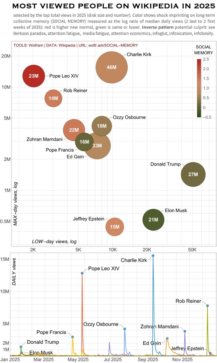
"Most-Viewed People on Wikipedia in 2025", my new article. Novel Social Memory wolfr.am/SOCIAL-MEMORY log ratio of post- to pre- catalyst event median Wikipedia pageviews, measuring how a catalyst event resets collective baseline attention. Comment If you know similar measures.
1
2
176
2 Dec 2025
⚛️ In 𝐫𝐢𝐯𝐞𝐫 𝐦𝐨𝐝𝐞𝐥 of 𝐛𝐥𝐚𝐜𝐤 𝐡𝐨𝐥𝐞𝐬 space itself flows...
River of space falls into black hole at Newtonian escape velocity, hitting light speed at horizon. Newton particle-grid with Wolfram differential equations gives a qualitative proxy for the visual:
🔴 Wolfram code & article: lnkd.in/dp6gk2gK
ABSTRACT excerpt: "The river model of black holes":
"The river model is mathematically sound, yet simple enough that the basic picture can be understood by non-experts. In the river model, space itself flows like a river through a flat background, while objects move through the river according to the rules of special relativity. In a spherical black hole, the river of space falls into the black hole at the Newtonian escape velocity, hitting the speed of light at the horizon. Inside the horizon, the river flows inward faster than light, carrying everything with it."
4
181
23 Sep 2025
How-to "see" 4th dimension in simple steps:
...using 𝐟𝐚𝐦𝐢𝐥𝐢𝐚𝐫 𝐨𝐛𝐣𝐞𝐜𝐭𝐬. 1️⃣ This 4D object = donut;
2️⃣ Cut typical 3D donut across its tube;
3️⃣ The shape of the cut is usual 2D circle;
4️⃣ Generalize by 1: cut 4D donut and get 3D shapes at the cut.
Which is similar to the red tubes in video. Those red tubes are shape of cuts when our familiar 3D space slices 4D donut. And they are similar to our typical 3D donuts!
What's your favorite application of higher dimensions?
TREFOIL KNOT & UNKNOT
Another stunning part in the video is gorgeous 𝐭𝐫𝐞𝐟𝐨𝐢𝐥 𝐤𝐧𝐨𝐭 falling apart into 2 separate rings and then reconnecting again into 𝐮𝐧𝐤𝐧𝐨𝐭 -- starting at t =12 seconds. I highly recommend to pause and slowly scroll through this structure. Its formation is analogical to how you twist 180° a paper band to make a Möbius strip. For details and code see:
🔴 Wolfram code & article: lnkd.in/eM5vES5x
APHANTASIA & ABSTRACT THINKING
𝐀𝐩𝐡𝐚𝐧𝐭𝐚𝐬𝐢𝐚 is the inability to visualize in the mind. Some people cannot form images in their thoughts, for example imagining an apple. Surprisingly people with aphantasia have ability to think of higher dimensions through the power of abstraction. Grasping very visual entities even with no ability to visualize. The mind is truly a mystery.
1
5
284
10 Sep 2025
𝓜𝐚𝐧𝐝𝐞𝐥𝐛𝐫𝐨𝐭 fractal encodes 𝓙𝐮𝐥𝐢𝐚 fractals.
Video: 𝐰𝐡𝐢𝐭𝐞 𝐝𝐨𝐭 in 𝓜 defines connectivity of 𝓙.
Both 𝓜 and 𝓙 fractals are defined as 𝐙 ↦ 𝐙² 𝐂
The difference? 𝓜 plots 𝐂, and 𝓙 plots 𝐙.
The white dot (parameter 𝐂) travels in 𝓜 set (corners) and the corresponding 𝓙 set is plotted in the center.
Thus: 𝓜𝐚𝐧𝐝𝐞𝐥𝐛𝐫𝐨𝐭 is an atlas for 𝓙𝐮𝐥𝐢𝐚.
It means each point 𝐂 (white dot) in 𝓜 set tells you the structure of the corresponding 𝓙 set. If white dot inside 𝓜 then 𝓙(𝐂) is one connected whole. If white dot outside 𝓜 then 𝓙(𝐂) shatters into dust. So the Mandelbrot works like a map: by scanning parameter space 𝐂, you can classify every possible Julia set for connectivity.
In Wolfram Language simplest code can plot these fractals. For example, functions below helped to make this video. Plot Mandelbrot:
MandelbrotSetPlot[]
or even create interactive apps for Julia:
Manipulate[JuliaSetPlot[Complex @@ p, PlotRange->1.5], {p, Locator}]
Despite few-symbol definition 𝐙 ↦ 𝐙² 𝐂 no finite computation exhausts an infinite fractal. Any algorithm gives only approximations. When facing infinitely intricate, infinitely explorable universes, the power of mathematical abstraction is to encode infinite in finite symbolic form. A few fun facts:
3
4
21
755
4 Sep 2025
𝐓𝐨𝐤𝐲𝐨 𝐬𝐮𝐛𝐰𝐚𝐲 is 99% on-time, world's best. But how lines can be shaped by 𝐄𝐝𝐨 𝐏𝐞𝐫𝐢𝐨𝐝 (1603–1868)?
Try to guess before reading further 👇 Each dot is a train (real data) ramping up to one of the world highest peak frequencies. Goes ~40m deep.
Tokyo's subway structure is quite complex. Japan has a law that land ownership extends to surface and underground. So land fee is due for subway construction. Unless... subway runs under the roads owned by the state or municipality, then underground is free for public interest. But the roads in Tokyo are made by filling the roads and waterways remaining from Edo period. They curve and run radially fitting the old Edo Castle. And that's how 1603–1868 shape modern subway.
𝘞𝘖𝘓𝘍𝘙𝘈𝘔 𝘢𝘳𝘵𝘪𝘤𝘭𝘦: community.wolfram.com/groups…
The whole data mining and visualization pipeline is done in Wolfram. Code base is quite small (see link above) due to large ~10K Wolfram function vocabulary and some packing neat algorithms like FindShortestTour used here.
1
4
327
3 Sep 2025
🟥 or 🟦 floats above the other?
This stereo illusion (𝐜𝐡𝐫𝐨𝐦𝐨𝐬𝐭𝐞𝐫𝐞𝐨𝐬𝐢𝐬) needs both eyes: close one and illusion is gone. 𝐁𝐨𝐢𝐝𝐬 or 𝐬𝐰𝐚𝐫𝐦 𝐢𝐧𝐭𝐞𝐥𝐥𝐢𝐠𝐞𝐧𝐜𝐞 type algorithm used in simulation - expand for tiny code👇
Wolfram Mathematica code (do you get what it does?):
n=3000;f:=(#/(.01 Sqrt[# . #]))&/@(x[[#]]-x)&;
x=Table[{Sin[a],-Cos[a]},{a,0.,2\[Pi],2\[Pi]/(n-1)}];
p=Table[Mod[i 1,n] 1,{i,n}];q=RandomInteger[{1,n},n];
Graphics[{Dynamic[Point[x=0.995 x 0.02 f[p]-0.01 f[q]]]}]
1
1
5
243
5 Jun 2025
𝐊𝐞𝐦𝐩𝐞'𝐬 𝐮𝐧𝐢𝐯𝐞𝐫𝐬𝐚𝐥𝐢𝐭𝐲 𝐭𝐡𝐞𝐨𝐫𝐞𝐦: There is a 𝐥𝐢𝐧𝐤𝐚𝐠𝐞 that signs your name. Proves a linkage exists to draw any algebraic planar curve. But to prove is NOT to design elegantly. Novel elegant method: community.wolfram.com/groups…
2
9
1,284
3 Jun 2025
𝐌𝐚𝐭𝐡 𝐃𝐞𝐭𝐞𝐜𝐭𝐢𝐯𝐞 wanted! Why recursion makes spirals?
a[n_] := Rescale[ a[n - 1] - GradientFilter[a[n - 1], 2] ]
1️⃣ 𝐚 --matrix or tensor of values ∈ [0, 1]
2️⃣ 𝐑𝐞𝐬𝐜𝐚𝐥𝐞 --keeps 𝐚 values ∈ [0, 1]
3️⃣ 𝐆𝐫𝐚𝐝𝐢𝐞𝐧𝐭𝐅𝐢𝐥𝐭𝐞𝐫 --discrete data gradient
3
9
38
2,008
3 Jun 2025
𝐖𝐨𝐥𝐟𝐫𝐚𝐦 code is very short:
𝕒[1] = RandomReal[1, 20 {1, 1, 1}];
𝕒[n_] := 𝕒[n] = Rescale[𝕒[n - 1] - GradientFilter[𝕒[n - 1], 2]]
Manipulate[𝕒[k]^10 // Image3D, {k, 1, 700, 1}]
Full original discussion by 𝐒𝐢𝐦𝐨𝐧 𝐖𝐨𝐨𝐝𝐬:
community.wolfram.com/groups…
5
201
3 Jun 2025
In the video this recursion is applied many times to a 3D table of values, shown as 3D image. 𝐒𝐭𝐚𝐛𝐥𝐞 𝐬𝐩𝐢𝐫𝐚𝐥𝐬 𝐞𝐦𝐞𝐫𝐠𝐞. Video runs evolution backwards to the initial random values, and then forward in time with slightly different visualization technique.
3
180
16 Apr 2025
𝐃𝐞𝐥𝐚𝐮𝐧𝐚𝐲 🔲 & 𝐕𝐨𝐫𝐨𝐧𝐨𝐢 🟦 meshes are DUALS of each other. 𝘤𝘰𝘳𝘳𝘦𝘴𝘱𝘰𝘯𝘥𝘪𝘯𝘨 🔲 & 🟦 edges are ⊥. 🔲 vertices <=> 🟦 cells. 🔲 triangles <=> 🟦 vertices. CODE: community.wolfram.com/groups…
1
5
28
1,916