Acá va el código de R library(shiny) library(bslib) library(dplyr) library(readr) library(sf) library(spdep) library(leaflet) library(DT) library(stringr) library(tibble) # Exploratory spatial autocorrelation for Delitos 2025. # This does not create property-level features. It aggregates incidents to a # hex grid and checks whether counts cluster spatially. BASE_DIR <- "C:/Users/sixto/Documents/CCA_Plusvalia" OUT_DIR <- "C:/Users/sixto/Documents/Codex/2026-06-14/files-mentioned-by-the-user-library/outputs/work/delitos_2025" dir.create(OUT_DIR, recursive = TRUE, showWarnings = FALSE) DELITOS_URL <- "data.buenosaires.gob.ar/data…" DELITOS_LOCAL <- "C:/Users/sixto/Documents/Codex/2026-06-14/files-mentioned-by-the-user-library/outputs/work/spatial_raw/delitos_2025.csv" DELITOS_CACHE <- if (file.exists(DELITOS_LOCAL)) DELITOS_LOCAL else file.path(OUT_DIR, "delitos_2025_raw.csv") BARRIOS_POPULARES_URL <- "data.buenosaires.gob.ar/data…" BARRIOS_POPULARES_LOCAL <- "C:/Users/sixto/Documents/Codex/2026-06-14/files-mentioned-by-the-user-library/outputs/work/spatial_raw/barrios_populares.csv" BARRIOS_POPULARES_CACHE <- if (file.exists(BARRIOS_POPULARES_LOCAL)) { BARRIOS_POPULARES_LOCAL } else { file.path(OUT_DIR, "barrios_populares.csv") } CABA_STREETS_SHP <- file.path(BASE_DIR, "callejero/calles.shp") WORK_CRS <- 3857 norm_txt <- function(x) { x <- toupper(as.character(x)) x <- iconv(x, from = "", to = "ASCII//TRANSLIT") x[is.na(x)] <- "" trimws(x) } scaled_coord <- function(x, axis = c("lon", "lat")) { axis <- match.arg(axis) x_chr <- gsub(",", ".", as.character(x), fixed = TRUE) x_chr <- vapply(x_chr, function(v) { if (is.na(v) || !grepl("^-?\\d \\.\\d \\.", v)) return(v) sign <- if (startsWith(v, "-")) "-" else "" parts <- strsplit(sub("^-", "", v), "\\.")[[1]] paste0(sign, parts[1], ".", paste(parts[-1], collapse = "")) }, character(1)) x <- suppressWarnings(as.numeric(x_chr)) if (all(is.na(x))) return(x) limit <- if (axis == "lon") 180 else 90 for (div in c(10, 100, 1000, 10000, 100000, 1000000, 10000000)) { x <- ifelse(!is.na(x) & abs(x) > limit & abs(x / div) <= limit, x / div, x) } x } read_delitos <- function(force = FALSE) { cache_path <- DELITOS_CACHE if (force || !file.exists(cache_path)) { cache_path <- file.path(OUT_DIR, "delitos_2025_raw.csv") download.file(DELITOS_URL, cache_path, mode = "wb", quiet = TRUE) } header <- readLines(cache_path, n = 1, warn = FALSE, encoding = "UTF-8") delim <- if (str_count(header, ";") > str_count(header, ",")) ";" else "," raw <- read_delim( cache_path, delim = delim, show_col_types = FALSE, col_types = cols(.default = col_character()), locale = locale(encoding = "UTF-8") ) names(raw) <- tolower(gsub("-", "_", names(raw))) raw |> mutate( tipo_norm = norm_txt(tipo), subtipo_norm = norm_txt(subtipo), uso_arma_norm = norm_txt(uso_arma), uso_moto_norm = norm_txt(uso_moto), barrio_norm = norm_txt(barrio), lon = scaled_coord(longitud, axis = "lon"), lat = scaled_coord(latitud, axis = "lat"), cantidad_num = suppressWarnings(as.numeric(cantidad)), cantidad_num = ifelse(is.na(cantidad_num), 1, cantidad_num), grupo = case_when( str_detect(tipo_norm, "HOMICIDIO") ~ "Homicidios", str_detect(tipo_norm, "^ROBO") ~ "Robos", str_detect(tipo_norm, "^HURTO") ~ "Hurtos", TRUE ~ "Otros" ) ) |> filter( !is.na(lon), !is.na(lat), between(lon, -59, -58), between(lat, -35, -34) ) |> st_as_sf(coords = c("lon", "lat"), crs = 4326, remove = FALSE) |> st_transform(WORK_CRS) } read_barrios_populares <- function(force = FALSE) { cache_path <- BARRIOS_POPULARES_CACHE if (force || !file.exists(cache_path)) { cache_path <- file.path(OUT_DIR, "barrios_populares.csv") download.file(BARRIOS_POPULARES_URL, cache_path, mode = "wb", quiet = TRUE) } bp <- read_delim( cache_path, delim = ",", show_col_types = FALSE, col_types = cols(.default = col_character()), locale = locale(encoding = "UTF-8") ) names(bp) <- tolower(names(bp)) if (!"geometry" %in% names(bp)) return(NULL) st_as_sf(bp, wkt = "geometry", crs = 4326) |> st_make_valid() |> st_transform(WORK_CRS) } get_caba_boundary <- function() { st_read(CABA_STREETS_SHP, quiet = TRUE) |> st_transform(WORK_CRS) |> st_geometry() |> st_buffer(180) |> st_union() |> st_as_sf() |> st_make_valid() } make_hex_counts <- function(delitos, boundary, selected_groups, hex_size) { d <- delitos |> filter(.data$grupo %in% selected_groups) hex <- st_make_grid(boundary, cellsize = hex_size, square = FALSE) |> st_as_sf() |> mutate(hex_id = row_number()) |> st_filter(boundary, .predicate = st_intersects) |> st_make_valid() if (nrow(d) == 0) { hex$count <- 0 return(hex) } joined <- st_join(d, hex, join = st_within) counts <- joined |> st_drop_geometry() |> filter(!is.na(hex_id)) |> group_by(hex_id) |> summarise(count = sum(cantidad_num, na.rm = TRUE), .groups = "drop") hex |> left_join(counts, by = "hex_id") |> mutate(count = ifelse(is.na(count), 0, count)) } run_moran <- function(hex_counts) { nb <- poly2nb(hex_counts, queen = TRUE) lw <- nb2listw(nb, style = "W", zero.policy = TRUE) x <- hex_counts$count global <- moran.test(x, lw, zero.policy = TRUE) local <- localmoran(x, lw, zero.policy = TRUE) x_mean <- mean(x, na.rm = TRUE) lag_x <- lag.listw(lw, x, zero.policy = TRUE) lag_mean <- mean(lag_x, na.rm = TRUE) hex_counts |> mutate( lag_count = lag_x, local_i = local[, "Ii"], local_p = local[, "Pr(z != E(Ii))"], lisa_cluster = case_when( local_p > 0.05 ~ "No significativo", count >= x_mean & lag_count >= lag_mean ~ "High-High", count <= x_mean & lag_count <= lag_mean ~ "Low-Low", count >= x_mean & lag_count <= lag_mean ~ "High-Low", count <= x_mean & lag_count >= lag_mean ~ "Low-High", TRUE ~ "No significativo" ), moran_i = unname(global$estimate[["Moran I statistic"]]), moran_p = global$p.value, expected_i = unname(global$estimate[["Expectation"]]) ) } delitos_all <- read_delitos(force = FALSE) barrios_populares <- read_barrios_populares(force = FALSE) caba_boundary <- get_caba_boundary() ui <- page_sidebar( title = "Autocorrelacion espacial - Delitos 2025", theme = bs_theme(version = 5, bootswatch = "litera"), sidebar = sidebar( width = 330, checkboxGroupInput( "grupo", "Grupo", choices = c("Homicidios", "Robos", "Hurtos", "Otros"), selected = "Robos" ), selectInput( "hex_size", "Tamano hexagono", choices = c("500 m" = 500, "750 m" = 750, "1000 m" = 1000, "1500 m" = 1500), selected = 750 ), checkboxInput("show_bp", "Mostrar barrios populares", value = TRUE), actionButton("run", "Actualizar Moran / LISA"), hr(), tags$p( class = "small text-muted", "Moran se calcula sobre conteos agregados por hexagono. Para homicidios conviene usar hexagonos mas grandes porque son pocos eventos." ) ), navset_tab( nav_panel("LISA mapa", br(), leafletOutput("lisa_map", height = 720)), nav_panel("Moran global", br(), verbatimTextOutput("global_moran")), nav_panel("Tabla hex", br(), DTOutput("hex_table")) ) ) server <- function(input, output, session) { moran_layer <- eventReactive(input$run, { hex_counts <- make_hex_counts( delitos = delitos_all, boundary = caba_boundary, selected_groups = input$grupo, hex_size = as.numeric(input$hex_size) ) run_moran(hex_counts) }, ignoreInit = FALSE) output$lisa_map <- renderLeaflet({ x <- moran_layer() validate(need(nrow(x) > 0, "Sin hexagonos.")) x4326 <- st_transform(x, 4326) bp4326 <- if (inherits(barrios_populares, "sf")) st_transform(barrios_populares, 4326) else NULL pal_lisa <- colorFactor( palette = c( "High-High" = "#d00000", "Low-Low" = "#1d4ed8", "High-Low" = "#f97316", "Low-High" = "#22c55e", "No significativo" = "#d1d5db" ), domain = c("High-High", "Low-Low", "High-Low", "Low-High", "No significativo") ) m <- leaflet(x4326, options = leafletOptions(preferCanvas = TRUE)) |> addProviderTiles(providers$CartoDB.Positron) |> addPolygons( fillColor = ~pal_lisa(lisa_cluster), fillOpacity = ~ifelse(lisa_cluster == "No significativo", 0.18, 0.62), color = "#ffffff", weight = 0.4, popup = ~paste0( "<b>Cluster:</b> ", lisa_cluster, "<br>", "<b>Count:</b> ", count, "<br>", "<b>Lag count:</b> ", round(lag_count, 2), "<br>", "<b>Local I:</b> ", round(local_i, 4), "<br>", "<b>p:</b> ", signif(local_p, 3) ) ) |> addLegend(position = "bottomright", pal = pal_lisa, values = ~lisa_cluster, title = "LISA") if (isTRUE(input$show_bp) && inherits(bp4326, "sf") && nrow(bp4326) > 0) { m <- m |> addPolygons( data = bp4326, fillColor = "#7b2cbf", fillOpacity = 0.08, color = "#5a189a", weight = 1.1, label = ~paste0(nombre, " | ", tipo) ) } m }) output$global_moran <- renderPrint({ x <- moran_layer() cat("Grupo:", paste(input$grupo, collapse = ", "), "\n") cat("Hex size:", input$hex_size, "m\n") cat("Hexagonos:", nrow(x), "\n") cat("Eventos agregados:", sum(x$count, na.rm = TRUE), "\n\n") cat("Global Moran's I:", round(unique(x$moran_i)[1], 5), "\n") cat("Expected I:", round(unique(x$expected_i)[1], 5), "\n") cat("p-value:", signif(unique(x$moran_p)[1], 5), "\n\n") cat("Interpretacion rapida:\n") if (unique(x$moran_p)[1] <= 0.05 && unique(x$moran_i)[1] > 0) { cat("- Hay autocorrelacion espacial positiva: los conteos se agrupan.\n") } else if (unique(x$moran_p)[1] <= 0.05 && unique(x$moran_i)[1] < 0) { cat("- Hay autocorrelacion negativa: patron tipo dispersion/alternancia.\n") } else { cat("- No hay evidencia fuerte de autocorrelacion global con este grid/filtro.\n") } }) output$hex_table <- renderDT({ x <- moran_layer() |> st_drop_geometry() |> arrange(local_p) datatable( x |> select(hex_id, count, lag_count, local_i, local_p, lisa_cluster, moran_i, moran_p), rownames = FALSE, options = list(pageLength = 25, scrollX = TRUE) ) }) } shinyApp(ui, server)

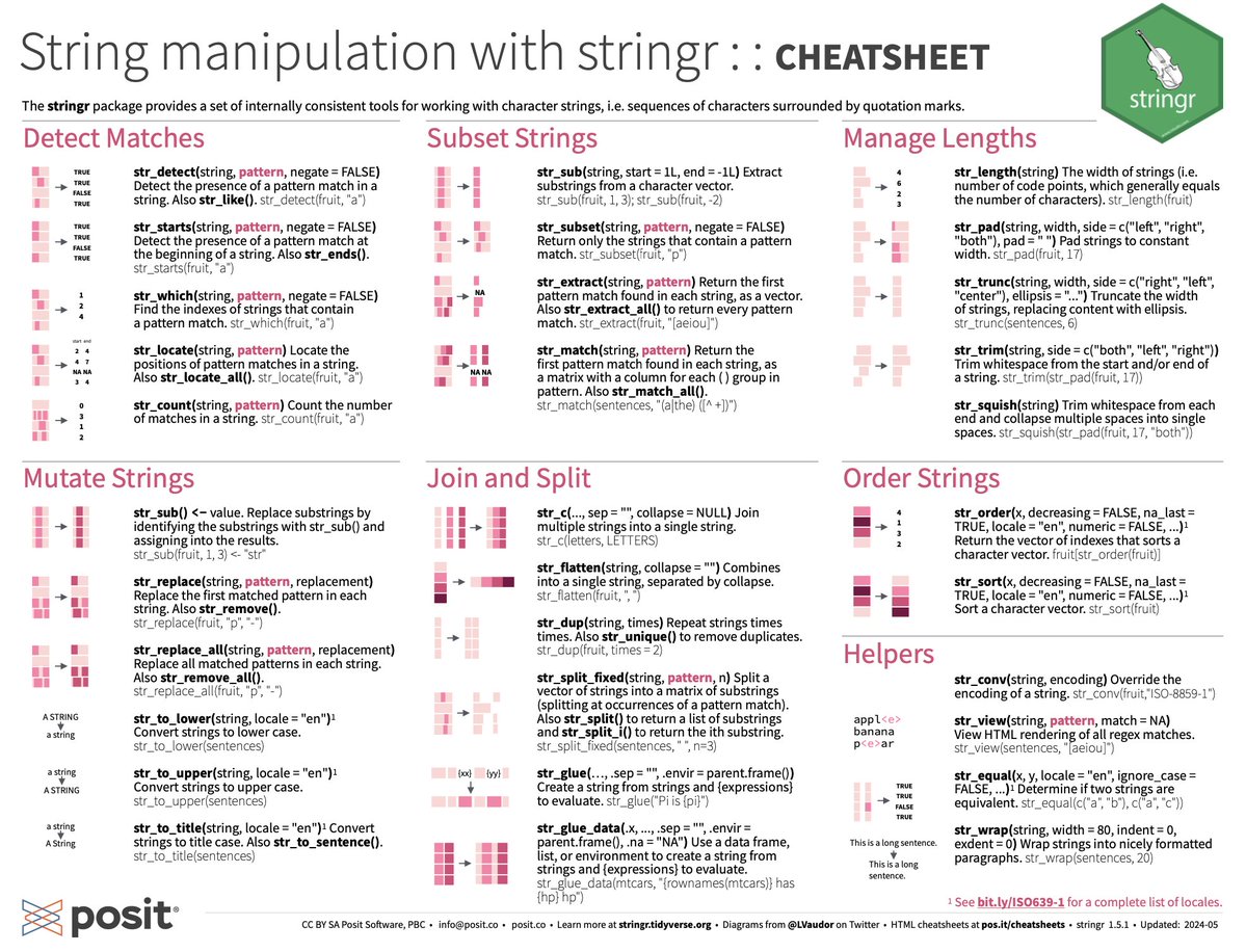
String manipulation is a critical daily task for bioinformaticians. Here is a cheatsheet using stringr: rstudio.github.io/cheatsheet… I probably use stringr::str_replace() once every other day... to clean up metadata (of course!) #rstats

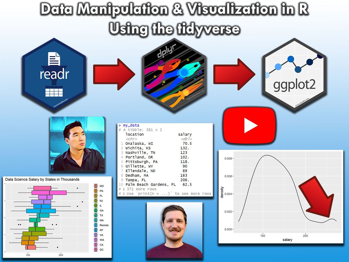
The tidyverse packages are perhaps the biggest advantage of the R programming language. To help you master them, I've created a video where I explain these powerful tools in practice. The example in this video is based on a data science salaries data set. To handle these data, I use: ✅ readr to import data ✅ stringr to manipulate character strings ✅ dplyr to manipulate data ✅ ggplot2 to visualize data Check out the video: youtube.com/watch?v=2PI0N_F0… The video is the result of a collaboration with the "Data Professor" Chanin Nantasenamat. The Data Professor YouTube channel offers videos on a wide range of data science topics, and I highly recommend checking it out: youtube.com/@DataProfessor Thanks again to Chanin for this great collaboration! This video also serves as a teaser for my online course on "Data Manipulation in R Using dplyr & the tidyverse." Take a look here for more details: statisticsglobe.com/online-c… #VisualAnalytics #datavis #RStats #DataAnalytics #tidyverse

✅ Complete R Programming Roadmap in 2 Months 📅 Month 1: Strong R Foundations 🔹 Week 1: R Basics & Environment - What is R and where it is used (analytics, statistics, ML) - Install R and RStudio - Variables, data types (numeric, character, logical) - Vectors, lists, matrices - Basic operations ✅ Outcome: You can write basic R code and understand data structures 🔹 Week 2: Data Handling & dplyr - Data frames and tibbles - dplyr basics: select(), filter(), mutate() - arrange() group_by() and summarise() - Import CSV using read.csv() ✅ Outcome: You can clean and transform datasets 🔹 Week 3: Data Visualization - Introduction to ggplot2 - Bar charts, line charts, scatter plots - Aesthetics (aes) - Themes and customization ✅ Outcome: You can visualize insights clearly 🔹 Week 4: Data Cleaning & Practice - Handling missing values (NA) - String manipulation (stringr) - Removing duplicates - Practice on real datasets ✅ Outcome: You prepare real-world clean datasets 📅 Month 2: Analytics Advanced R 🔹 Week 5: Statistics in R - Mean, median, standard deviation - Correlation and covariance - Hypothesis testing (t-test) - Basic statistical functions ✅ Outcome: You understand data scientifically 🔹 Week 6: Advanced Data Manipulation - Joins in R (merge, dplyr joins) - tidyr - Data reshaping (pivot_longer, pivot_wider) - Pipes (%>%) ✅ Outcome: You handle complex datasets easily 🔹 Week 7: Machine Learning Basics - Linear regression - Classification basics - Train-test split - Intro to caret ✅ Outcome: You can build basic ML models 🔹 Week 8: Project Interview Prep - Build a project (sales / HR dataset) - Use R Markdown - Create insights visualizations - Practice interview questions ✅ Outcome: You are job-ready in R 🧠 Practice Platforms - Kaggle (datasets notebooks) - DataCamp (R courses) - HackerRank (basic challenges) Double Tap ❤️ For Detailed Explanation of Each Topic

stringr::str_trim() -- kills invisible whitespace tidyr::separate() -- splits messy combined columns These aren't glamorous. They're survival tools.

Full video: youtu.be/d9ZPxyWfA3I Sign up for Stringr here: stringr.com/join/H68BE8 *use code H68BE8 at signup for $10, when you make your first sale.

5 Signs You’re Becoming a More Efficient Data Wrangler in R: 1️⃣ You handle NA values like a pro. Missing values used to cause panic, but now you know exactly how to deal with them—whether it’s using na.omit(), tidyr::fill(), or writing your own imputation function based on the context of your data. 2️⃣ You know the power of regular expressions. When it comes to text manipulation, you no longer fear stringr. Instead of manually cleaning strings, you use regex patterns to find, replace, or extract text efficiently, saving time and reducing errors. 3️⃣ You think about memory efficiency. You’ve started considering the size of your data frames and how to optimize them. Converting character vectors to factors, using data.table for large data sets, and clearing memory when it’s no longer needed are part of your workflow. 4️⃣ You work with date and time effortlessly. Instead of struggling with date formats, you’re comfortable using the lubridate package. Parsing, formatting, and performing calculations on date and time data have become second nature to you. 5️⃣ You understand the importance of reproducibility. You no longer write code that only works on your machine. Using R Markdown to document your work, organizing your project folders, and creating scripts that can be run by others without hassle are now part of your habits. For more data science tips, join my free email newsletter. Take a look here for more details: statisticsglobe.com/newslett… #RStats #DataAnalytics #datascienceenthusiast #Python #R #pythoncode

Why are you such a dumb fucking idiot? Wasting more money while people can't afford basics. Rhttps://www.rawstory.com/stringr/house-gop-investigating-bad-bunny/

The tidyverse packages are perhaps the biggest advantage of the R programming language. To help you master them, I've created a video where I explain these powerful tools in practice. The example in this video is based on a data science salaries data set. To handle these data, I use: ✅ readr to import data ✅ stringr to manipulate character strings ✅ dplyr to manipulate data ✅ ggplot2 to visualize data Check out the video: youtube.com/watch?v=2PI0N_F0… The video is the result of a collaboration with the "Data Professor" Chanin Nantasenamat. The Data Professor YouTube channel offers videos on a wide range of data science topics, and I highly recommend checking it out: youtube.com/@DataProfessor Thanks again to Chanin for this great collaboration! This video also serves as a teaser for my online course on "Data Manipulation in R Using dplyr & the tidyverse." Check out this link for more details: statisticsglobe.com/online-c… #RStats #Data #Python #Rpackage #datascienceenthusiast #pythonprogramming #VisualAnalytics

purrrとstringrがアップデート。 tidyverse.org/blog/ #R言語 #rstatsj

Oh, that's why I got urgent requests, from Stringr, to go down to the library to shoot video. Told them I had plans to shoot video of music (which was true.) If I want dangerous, I'll stay up in Lanier.

5 Signs You’re Becoming a More Efficient Data Wrangler in R: 1️⃣ You handle NA values like a pro. Missing values used to cause panic, but now you know exactly how to deal with them—whether it’s using na.omit(), tidyr::fill(), or writing your own imputation function based on the context of your data. 2️⃣ You know the power of regular expressions. When it comes to text manipulation, you no longer fear stringr. Instead of manually cleaning strings, you use regex patterns to find, replace, or extract text efficiently, saving time and reducing errors. 3️⃣ You think about memory efficiency. You’ve started considering the size of your data frames and how to optimize them. Converting character vectors to factors, using data.table for large data sets, and clearing memory when it’s no longer needed are part of your workflow. 4️⃣ You work with date and time effortlessly. Instead of struggling with date formats, you’re comfortable using the lubridate package. Parsing, formatting, and performing calculations on date and time data have become second nature to you. 5️⃣ You understand the importance of reproducibility. You no longer write code that only works on your machine. Using R Markdown to document your work, organizing your project folders, and creating scripts that can be run by others without hassle are now part of your habits. For more data science tips, join my free email newsletter. Learn more by visiting this link: eepurl.com/gH6myT #rstudioglobal #RStats #DataScience #Statistics

TRIGGER WARNING: Gun violence A man drove his vehicle through the front doors of a Church of Jesus Christ of Latter-day Saints and shot at least 10 people, killing one of them, local police said on Sunday, September 28. The shooter got out of his vehicle firing an assault-style weapon, Grand Blanc Chief of Police William Renye said. He added that hundreds of people were in the church, which was set on fire when the vehicle smashed into it. Authorities believe they will find additional victims in the ruins, the chief said. Police did not immediately release the name of the suspect, who died at the scene in an exchange of gunfire with two officers who rushed to the church, the chief said. The Church of Jesus Christ of Latter-day Saints is informally known as the Mormons. | via Reuters Video courtesy: stringr . com via Reuters

{stringr} update: #RStats #Tidyverse New `str_to_camel()`, `str_to_snake()`, and `str_to_kebab()` for changing "programming" case (@​librill, #573). github.com/tidyverse/stringr…

The tidyverse packages are perhaps the biggest advantage of the R programming language. To help you master them, I've created a video where I explain these powerful tools in practice. The example in this video is based on a data science salaries data set. To handle these data, I use: ✅ readr to import data ✅ stringr to manipulate character strings ✅ dplyr to manipulate data ✅ ggplot2 to visualize data Check out the video: youtube.com/watch?v=2PI0N_F0… The video is the result of a collaboration with the "Data Professor" Chanin Nantasenamat. The Data Professor YouTube channel offers videos on a wide range of data science topics, and I highly recommend checking it out: youtube.com/@DataProfessor Thanks again to Chanin for this great collaboration! This video also serves as a teaser for my online course on "Data Manipulation in R Using dplyr & the tidyverse." For more information, visit this link: statisticsglobe.com/online-c… #ggplot2 #statisticsclass #R4DS #RStats #DataVisualization #Rpackage

String manipulation is a critical daily task for bioinformaticians. Here is a cheatsheet using stringr: rstudio.github.io/cheatsheet… I probably use stringr::str_replace() once every other day... to clean up metadata (of course!) #rstats

Cliente pressionando, banco legado quebrando, Power BI travando? Use dplyr tidyr stringr e resolva tudo com clareza. 📊 Tidyverse: salvando projetos desde sempre. Você não precisa de mais dados. Precisa de dados mais inteligentes. rseis.com.br #RStats #tidyverse

eu morro e não aprendo todas as funções do tidyverse o {stringr} tem um uma função, `str_pad`, que fixa o tamanho minimo de uma string e preenche ele com algum caracter. Isso é MTO UTIL quando a gente ler tabela em excel onde o excel força numerico em coluna de id

A dúvida da Fernanda Kelly era: Como adicionar sufixo ao nome das colunas no tidyverse? 💡 Solução do @juliotrecenti: Use rename_with() stringr::str_c() Prático e legível! 📌 github.com/orgs/curso-r/disc… #RStats #tidyverse #dplyr #CursoR #DataScience