
the ART of TRADING
Joined September 2017
- Tweets 5,508
- Following 517
- Followers 3,433
- Likes 4,746
1,092 Photos and videos


PL retweeted

OpenAI’s financials have leaked, showing $21 billion in losses against $13 billion in revenue, per Fortune
100
229
2,370
678,274
if you look at what is working best... its the obvious "low IQ" darling stocks that are on everyone's mind, from pullback like pivots: semis -> $AMD $INTC $ARM $MRVL / adjacent $DELL ai hpc: $NBIS .. $SPCX ..
turnaround in optics but no amazing follow through and no super clean setup. $LITE actionable few days ago but choppy character.. $AXTI clean trader way up and down, 50day U&R not my kind of setup but clean confluence 6/12 5min ORB / 2PDH with 50day reclaim off to races..
post catalyst flags are not working as well, and not clean traders generally.. some recent best examples $VECO after few shakeouts.. $AMBQ no follow through..
$GH example of nice pattern but rando stock not in a key market group..
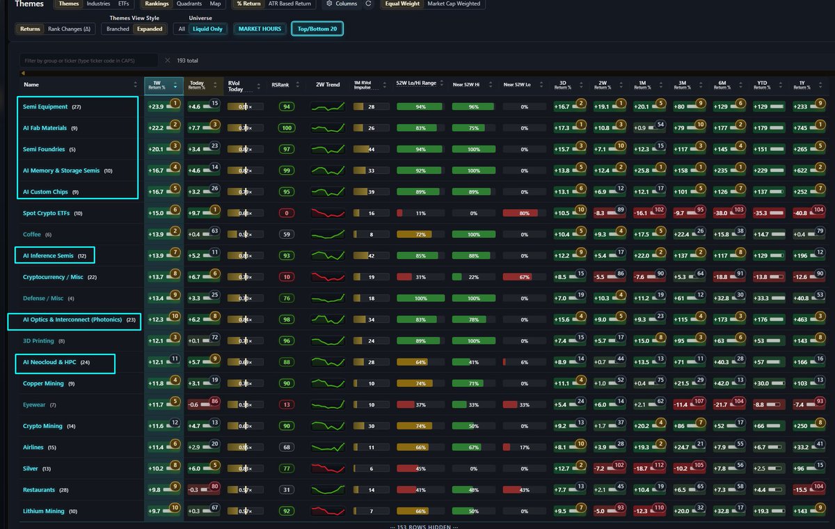
you can look at relative themes/groups performance wiht alot of "semi" (inference/testing/equipment/custom chips) and AI HPC are the ones that have maintained RS vs market throughout..
Crypto and Silver joining with "bottom bounce" type moves more recently, from a general strategy stand point these are lower grade as highest RS "wins" as a ranking principle during shallower corrections as we've had lately with $QQQ to the 50day MA.
market "higher lowed" at the 50day faster than expected, leaders off to races without much of a pivot "faster than expected" ... burden of proof back on the bears/shorts at this point.
1
11
1,463
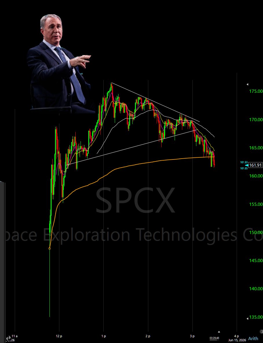
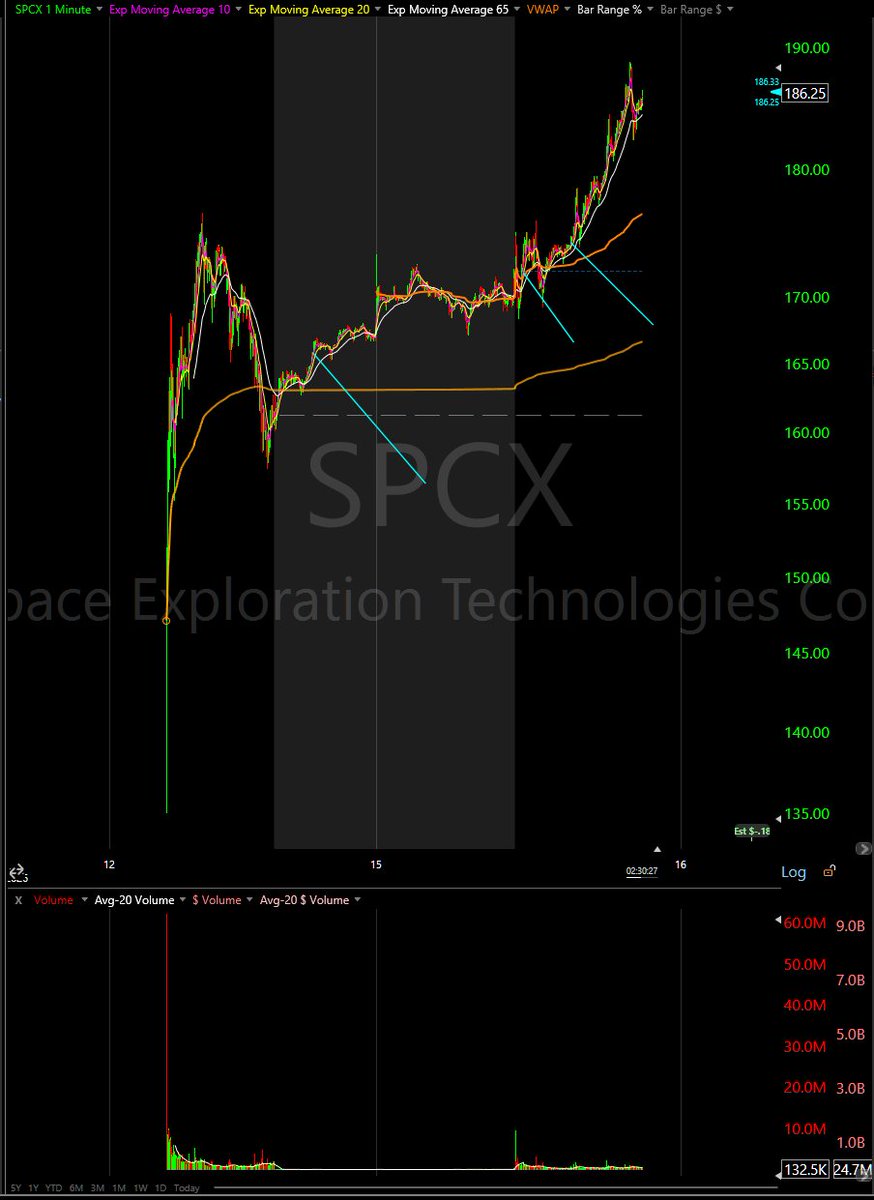
$SPCX following $CRCL template pretty closely.. close at vwap (nomansland) day 1 after strong day but undercut of vwap into close.. up pre market follow through D2. 10 odd 2x levered ETFs on $SPCX.. options tuesday.. indices additions.. "the world" wants you to buy this stock it seems lol.. and its acting like it.. roundtripped decent gain into a loss D1 even tho D1 performance was well within template.. afterhours D1 or VWAP curl today as D2 valid setups today.. gap up tomorrow first decision pt on exit, wiht obviously any flag-like structure on daily actionable as a long..
with ETFs and index related buying, look at itnraday surf of MAs for clues...


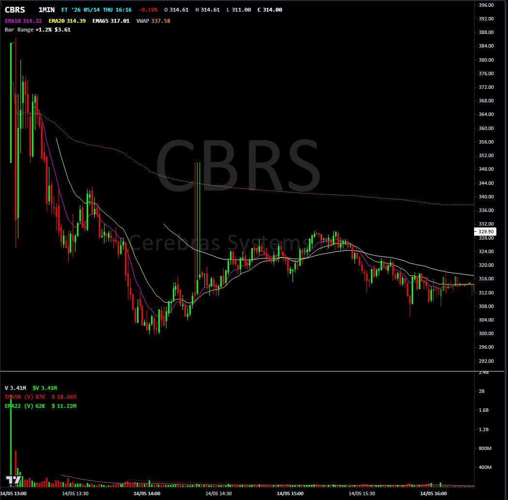
memorable recent IPO day 1s:
$CRCL 1 year 7 days ago exactly [crypto]
$BLSH (Bearish) 2025-08-13 [crypto]
$CRWV 2025-03-18
$CRBS 2026-05-14


1
9
1,391
PL retweeted

Jun 14
I'm doing one quick targeted pass so I can give you the exact answer rather than hand-waving
66
68
1,514
91,383
This is contradicts mainstream portfolio theory which is rooted in mean-variance optimisation and Sharpe ratio type stuff.
Instead you optimise for your actual intended end state, optimal compounded return growth aka optimal log growth and use information theory maths to assess how well your a specific strategy “compresses information surprise” vs a baseline you’re comparing against.
Compression in information surprise is effectively a measure of prediction improvement aka increased edge in your strategy (if any).
Sharpe and mean-variance doesn’t handle practical realities of trading/investing well:
- distribution skews
- fat-tails
- path-dependency as a property of your strategy, not “overfitting” !
- regime-sensitivity of your strategy
So with mean variance maths you end up adding crude “patches” and dirty heuristics to deal with these realities.
If you apply information theory you have a fundamental first principles approach to modelling predictive power.
Credits Kelly 1956; Claude Shannon; KL divergence dudes; Thomas M Cover; Stiffelman (2026, arXiv)
See screenshot. Trading portfolio optimisation is about COMPOUNDED return growth not arithmetic return growth, for obvious reasons. If you lose all your chips, you can’t bet.
Log(0) = negative infinity.
So that’s why we use log return growth in Kelly sizing not arithmetic.
Typical expectancy formula EV=p(win) (1-p)*loss becomes a naive abstraction. You only realise it’s naïveté when you confront risk of ruin modelling.
Optimal trading portfolio allocation, ie allocation of position weights across a number of assets is given by
G(W) = term 1 - term 2 - term 3
Term (1)
the payoffs of the optimal set of return paths.
Think of it as
Optimal market “opportunity”/forward return distribution (it is never known or knowable in principle, but if only you could know it…
Term (2)
2nd term is the natural irreducible uncertainty of the optimal market opportunity distribution. (Hint: information entropy)
Term (3)
is how much your actual allocation differs from the optimal. Ie let’s say it the true optimal allocation is (20% to stock A, 80% to stock B).
And you are allocated 50,50. You can measure the “information loss” or edge loss from your allocation vs the optimum. (Hint: KL divergence).
Now, W* in H(W*) is the collection (vector) of position allocations that would maximize expected your COMPOUNDED account growth if you knew the true joint market’s return distribution.
That is the theoretical optimum. In reality you can never know W*.
That’s why an achievable PRACTICAL optimum is: how can we get as close as I can to W* without knowing the true distribution?
Crucially, in the equation above, which btw isn’t just made up but is deterministically derivable from Kelly Cover’s universal portfolio theory,
Your allocation / trading decisions only ever affect term 3. So optimisation problem reduces to optimising the KL divergence between your allocation to the true optimal allocation.
Re-formulation of portfolio return optimisation
In this way is breaking new ground, because it gives you an ordering principle/heuristic to use in your backtesting:
You can now evaluate the quality of your (backtested or realised) return distribution and the quality of your allocation in the same unit: log-growth / information bits.
Each factor/feature of the strategy has a “usefulness” score as given by its KL divergence.
You can use these scores to optimise sizing.
This enables you to calculate m a “practical optimum” :
What is the best position size to use on a setup that has a known historical return distribution GIVEN you know certain features of a the setup in advance.
1
2
1,065
See screenshot. Trading portfolio optimisation is about COMPOUNDED return growth not arithmetic return growth, for obvious reasons. If you lose all your chips, you can’t bet.
Log(0) = negative infinity.
So that’s why we use log return growth in Kelly sizing not arithmetic.
Typical expectancy formula EV=p(win) (1-p)*loss becomes a naive abstraction. You only realise it’s naïveté when you confront risk of ruin modelling.
Optimal trading portfolio allocation, ie allocation of position weights across a number of assets is given by
G(W) = term 1 - term 2 - term 3
Term (1)
the payoffs of the optimal set of return paths.
Think of it as
Optimal market “opportunity”/forward return distribution (it is never known or knowable in principle, but if only you could know it…
Term (2)
2nd term is the natural irreducible uncertainty of the optimal market opportunity distribution. (Hint: information entropy)
Term (3)
is how much your actual allocation differs from the optimal. Ie let’s say it the true optimal allocation is (20% to stock A, 80% to stock B).
And you are allocated 50,50. You can measure the “information loss” or edge loss from your allocation vs the optimum. (Hint: KL divergence).
Now, W* in H(W*) is the collection (vector) of position allocations that would maximize expected your COMPOUNDED account growth if you knew the true joint market’s return distribution.
That is the theoretical optimum. In reality you can never know W*.
That’s why an achievable PRACTICAL optimum is: how can we get as close as I can to W* without knowing the true distribution?
Crucially, in the equation above, which btw isn’t just made up but is deterministically derivable from Kelly Cover’s universal portfolio theory,
Your allocation / trading decisions only ever affect term 3. So optimisation problem reduces to optimising the KL divergence between your allocation to the true optimal allocation.
Re-formulation of portfolio return optimisation
In this way is breaking new ground, because it gives you an ordering principle/heuristic to use in your backtesting:
You can now evaluate the quality of your (backtested or realised) return distribution and the quality of your allocation in the same unit: log-growth / information bits.
Each factor/feature of the strategy has a “usefulness” score as given by its KL divergence.
You can use these scores to optimise sizing.
This enables you to calculate m a “practical optimum” :
What is the best position size to use on a setup that has a known historical return distribution GIVEN you know certain features of a the setup in advance.
3
1,895
PL retweeted

Jun 13
*ANTHROPIC: RECEIVED DIRECTIVE FROM U.S. GOVERNMENT TODAY AT 5:21PM, LETTER DID NOT PROVIDE SPECIFIC DETAILS OF ITS NATIONAL SECURITY CONCERN
*ANTHROPIC: OUR UNDERSTANDING IS THAT U.S. GOVT BELIEVES IT HAS BECOME AWARE OF A METHOD OF BYPASSING, OR “JAILBREAKING” FABLE 5
*ANTHROPIC: SUSPECT THAT PERFECT JAILBREAK RESISTANCE IS NOT CURRENTLY POSSIBLE FOR ANY MODEL PROVIDER
*ANTHROPIC- IF THIS STANDARD WAS APPLIED ACROSS THE INDUSTRY, IT WOULD ESSENTIALLY HALT ALL NEW MODEL DEPLOYMENTS FOR ALL FRONTIER MODEL PROVIDERS
5
7
83
11,233
Alpha is the first Greek letter. Omega is the last.
Our mind imagines experience in a linear fashion. Beginning to end.
However, “being” is a circle. Alpha and Omega on a circle is the same point.
We emerge out of source and instead of “completion”, through “difference” and experience we return to source, enriched by the journey.
The circle of being never ceases. It is ever present. It starts at infinite intelligence and returns to infinite intelligence, with limitations existing at varying degrees only in our awareness.
3
468
PL retweeted

Jun 12
Absolutely hilarious that $MRVL went down instantly AH yesterday after they announced that they hired the CFO of Adobe. Imagine having a management team so disliked that investors treat your executives like transferable liabilities LOL
10
3
102
11,323
PL retweeted

Jun 10
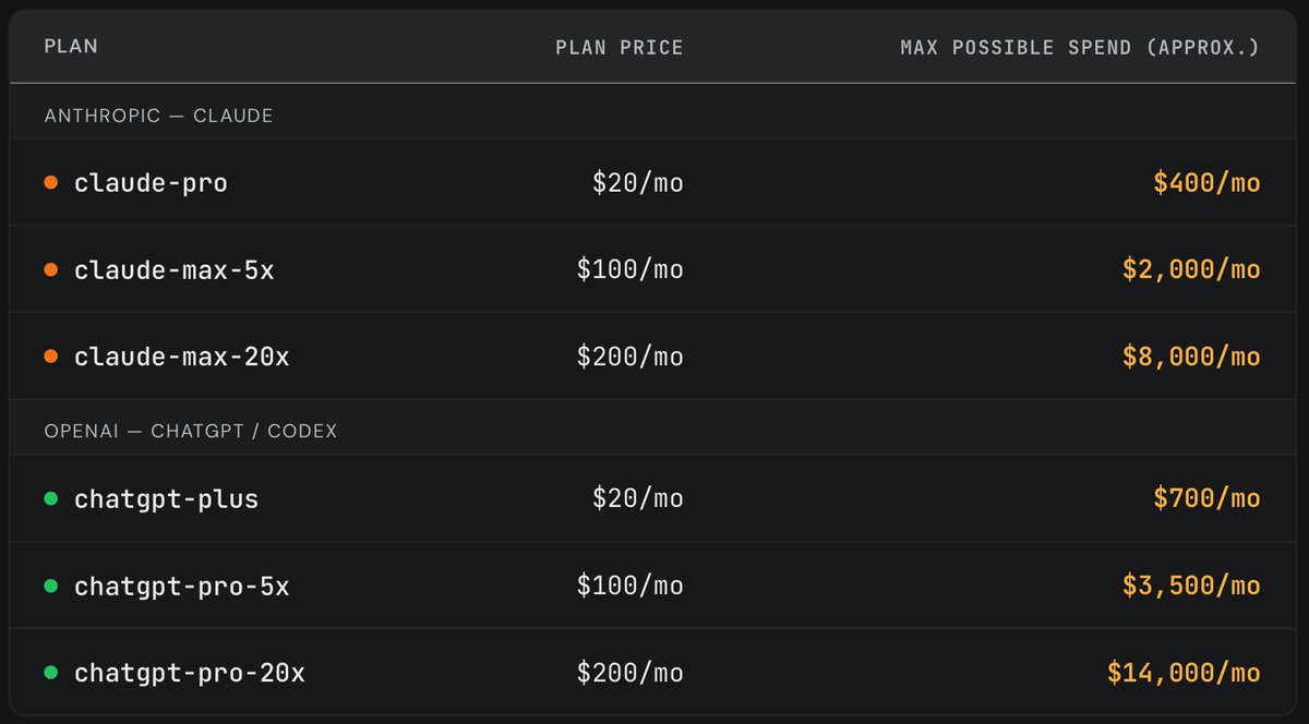
Recently, we purchased one of each Anthropic/OpenAI subscription plan and randomly ran long horizon coding tasks until we exhausted the weekly limit. It's widely believed that a $200/month plan maxes out at ~$2000/month worth of tokens (assuming API pricing). However, we found that the subscriptions are actually far more generous. (2/4)
201
586
6,120
3,515,848

