
May 31
This is Plateau’s problem
You dip the rings into soap, lift them out, and the film quietly organizes itself.
No equations are solved on paper, yet the shape that appears is the solution to a Calculus of variations problem:
Among all surfaces spanning the same boundary, it picks the one with minimal surface area.
#PlateausProblem #CalculusOfVariations #MinimalSurfaces #Catenoid #SoapFilmPhysics #GeometricOptimization
9
17
111
5,956
May 30
In Calculus of Variations, we give up the idea of only optimizing values and start optimizing geometries instead.
The unknown is not a single x. It is a whole curve/surface y(x). The object you are minimizing is usually not a simple formula that you can guess. It is an integral that judges the whole shape.
In our first lecture, we discuss the famous Brachistochrone problem. You choose two points, turn on gravity and ask a question which almost sounds too simple...which track will allow a bead to move from A to B in the minimum time?
At your first attempt, your instinct will lead you astray. It is not the straight line. It is not the drop hard then cruise sketch either. The winner turns out to be a cycloid...the curve a point on a rolling circle traces.
The track is the moving character in the animation. We begin with a flawed curve, perform gradient descent in curve-space, and observe the geometry change frame by frame as T[y] collapses to the brachistochrone.
Please see the comment below for the math breakdown.
#CalculusOfVariations #Brachistochrone #Cycloid #Physics #Optimization #Mathematics
9
44
310
23,226
Feb 14
Which Curve Wins the Race Under Gravity?
Calculus of Variations is what happens when you stop optimizing values and start optimizing geometries. The unknown isn’t a single x…it’s the whole curve y(x). And in higher dimensions, it’s the whole surface u(x,y). And the thing you’re minimizing usually isn’t a formula you can eyeball…it’s an integral that judges the entire shape.
For our first lecture, we look at the famous Brachistochrone problem. Fix two points, switch on gravity, and ask a question that sounds almost too simple…which track gets a bead from A to B in the least time?
Your intuition will betray you on the first try. It’s not the straight line. It’s not the drop hard then cruise sketch either. The winner is a cycloid…the curve traced by a point on a rolling circle.
In the animation, the track is the moving character. We start with an imperfect curve, run gradient descent in curve-space, and watch the geometry reshape frame by frame as T[y] collapses until it locks into the brachistochrone.
Here is the breakdown of the math.
Set coordinates so downhill is visually obvious without negatives. Put the start above the x-axis and the finish on it:
A = (0, H), B = (L, 0), with H > 0.
A track is a graph y = y(x) on x ∈ [0, L] with y(0) = H and y(L) = 0.
Physics from rest:
By energy conservation, height drop (H − y(x)) turns into speed,
v(x) = √(2g(H − y(x))).
Geometry gives the arc-length element,
ds = √(1 (y′(x))²) dx.
So the time element is just distance-over-speed:
dt = ds / v
= √(1 (y′)²) / √(2g(H − y)) · dx.
That makes the travel time a single object:
T[y] = ∫₀ᴸ √((1 (y′(x))²) / (2g(H − y(x)))) dx.
That’s the target. Not shortest path, not steepest drop. Minimize T[y].
Then we do an honest discrete-to-variational move: parameterize curves that hit the endpoints automatically, evaluate T[y] by quadrature on a fine grid, and run gradient descent in the coefficients to shrink T.
#CalculusOfVariations #Brachistochrone #Cycloid #ClassicalMechanics #Optimization #MathAnimation
7
32
286
22,933
27 Dec 2025
Lecture 4 on Calculus of Variations
You might wonder...If I’m optimizing a shape...a curve, a surface, a whole path, what does "take the derivative and set it to zero" even mean? Do I take the damn derivative with respect to a curve/surface? 🤔
In normal calculus the variable is a number x, so the reflex is clean...f′(x)=0. In calculus of variations the variable is a whole function...the geometry itself, like a curve y(x) (or a surface z(x,y)). So the derivative can’t be a single slope. It has to be a pointwise sensitivity, i.e. how the objective reacts to tiny local deformations.
You’re holding a whole shape, like a curve y(x). Your objective isn’t f(x) anymore, it’s a functional J[y], and as we've seen with our first there examples, usually an integral that depends on the entire curve (often through y and y’).
To talk about a “derivative”, you do the only thing that makes sense: you nudge the entire curve by a tiny amount and see how J changes. Pick a wiggle shape η(x). It’s not random...it’s any admissible deformation direction.
Admissible just means it obeys the constraints. If the endpoints are fixed, you force η(0)=η(1)=0 so the wiggle doesn’t move the endpoints. Then scale that wiggle by a small number ε and define the perturbed curve yε(x)=y(x) εη(x).
Now treat ε like the usual scalar in a Taylor expansion. As ε→0, J[y εη] expands as
J[y εη] = J[y] ε · (first-order term depending linearly on η) o(ε).
So the difference is
J[y εη] - J[y] = ε · (linear functional of η) o(ε).
For the standard integral of a Lagrangian problems, that linear functional can be written as an inner product with some function of x:
J[y εη] - J[y] = ε ∫ (δJ/δy)(x) η(x) dx o(ε).
That’s the definition-level meaning of δJ/δy: it’s the unique pointwise sensitivity function that makes this identity true for every admissible η. If δJ/δy is positive at some x, then choosing η negative there decreases J; if δJ/δy is negative there, pushing y upward locally decreases J. It’s literally a map along the curve saying push this way to go downhill.
Now translate “set the derivative to zero.”
At a minimizer y*, the first-order change must vanish for every admissible wiggle:
J[y* εη] − J[y*] = o(ε) for all η.
Plug in the expansion and the ε-term must be zero:
∫ (δJ/δy)(x) η(x) dx = 0 for all admissible η.
Here’s the crucial logic step: the only way an integral against every test function η can be zero is if the integrand itself is zero (in the usual sense used in analysis). So you get
δJ/δy = 0.
For the common case J[y]=∫ L(x, y, y’) dx, you can compute δJ/δy explicitly and it becomes the Euler–Lagrange expression
δJ/δy = ∂L/∂y − d/dx(∂L/∂y’).
So if you name the Euler–Lagrange residual as “left-hand side”
R(x) = ∂L/∂y − d/dx(∂L/∂y’),
then “set the derivative to zero” is exactly R(x)=0.
That’s why animation works so well. You don’t have to solve R=0 in one shot. You can evolve the curve in an artificial time τ by pushing it in the downhill direction:
∂y/∂τ = −R(y).
Where the residual is large, the curve moves a lot; as the residual drains toward zero, the motion dies out and the curve settles into an extremal.
In our animations, we start from an intentionally ugly curve/surface. Frame by frame the functional drops, the residual drains away, and the geometry relaxes into an extremal.
#CalculusOfVariations #EulerLagrange #FunctionalDerivative #GradientFlow #Optimization #MathAnimation
6
46
269
12,133
26 Dec 2025
In Lecture 3 of our Calculus of Variations series, we hand the steering wheel to light.
We don’t tell it how to bend. We only define what time costs.
We render a 2D refractive-index field n(x,y). A fan of rays launches from a source and curves through the gradient, shown as volumetric glow. Then we pin a start point and an end point and do the honest thing...run gradient descent in path-space on optical time, watching the straight path deform into the Fermat minimizer.
T (the optical travel time of a path) drops frame by frame, and n(y) sin θ along the converged ray stays almost flat.
Snell’s law isn’t an extra rule. It’s the constant of motion you can see. 👌🏾
See the math breakdown below
#CalculusOfVariations #FermatsPrinciple #SnellsLaw #GeometricOptics #Optimization #MathAnimation
2
22
148
7,117
26 Dec 2025
Lecture 1 was our first taste of what Optimizing a Geometry really means. We didn’t tune a number, we let an entire curve y(x) reshape until the travel-time functional collapsed into the brachistochrone.
Lecture 2 is the same move, just one dimension up. Now the unknown isn’t a curve...it’s a whole surface in 3D.
Fix two rigid rings in space, dip them in soap, and the film that forms is nature solving a variational problem: Minimize surface area subject to those boundary circles.
Your intuition will betray you again. The obvious bridge is a cylinder, but a cylinder wastes area. When you let the surface relax, it tightens, a neck forms, and the geometry settles toward the catenoid...a shape that looks engineered, but it’s just what minimizing the area functional forces.
In the animation we start from a fat surface and run gradient descent in surface-space. You watch the area of the surface drop frame by frame until the film locks into its minimal shape under the boundary constraint.
Pls see the comment below for the math breakdown.
#CalculusOfVariations #MinimalSurfaces #PlateauProblem #Catenoid #SoapFilm #MathAnimation
2
18
174
12,727
26 Dec 2025
Here is the breakdown of the math.
Set coordinates so downhill is visually obvious without negatives. Put the start above the x-axis and the finish on it:
A = (0, H), B = (L, 0), with H > 0.
A track is a graph y = y(x) on x ∈ [0, L] with y(0) = H and y(L) = 0.
Physics from rest:
By energy conservation, height drop (H − y(x)) turns into speed,
v(x) = √(2g(H − y(x))).
Geometry gives the arc-length element,
ds = √(1 (y′(x))²) dx.
So the time element is just distance-over-speed:
dt = ds / v
= √(1 (y′)²) / √(2g(H − y)) · dx.
That makes the travel time a single object:
T[y] = ∫₀ᴸ √((1 (y′(x))²) / (2g(H − y(x)))) dx.
That’s the target. Not shortest path, not steepest drop. Minimize T[y].
Then we do an honest discrete-to-variational move: parameterize curves that hit the endpoints automatically, evaluate T[y] by quadrature on a fine grid, and run gradient descent in the coefficients to shrink T.
The cycloid isn’t magic...it’s where the time functional keeps dragging you.
#CalculusOfVariations #Brachistochrone #Cycloid #ClassicalMechanics #Optimization #MathAnimation
1
4
36
3,840

26 Jan 2025
the solution of the Brachistochrone problem resulted in the development of the branch of mathematics called Calculus of Variations
#BrachistochroneProblem
#CalculusOfVariations
#Cycloid
2
207

17 Oct 2024
I am pleased to share that I have recently accepted invite to join the editorial board of Scientific reports.
@NaturePortfolio
#SciReports
#mechanics
#softmatter
#wavescattering
#elasticity
#geometry
#instabilities
#lattices
#stochastic
#calculusofvariations
#PDE
#metamaterials
8
452

23 Aug 2024
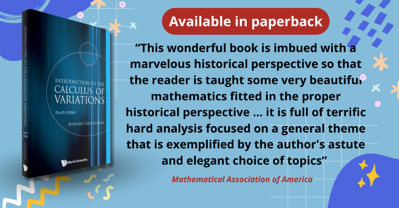
Unlock the power of optimization! Discover the calculus of variations and its applications in physics, engineering, economics, and biology. With detailed solutions and exercises, this guide is perfect for students and researchers! 📚
#calculusofvariations #mathematics
1
6
55
640,001

28 Jun 2024
#NextatBIRS Mathematical Analysis of Soft Matter, June 30 - July 5, 2024
birs.ca/event/24w5249
#ModernAppliedAnalysis #PartialDifferentialEquations #CalculusofVariations #OptimalControl #Optimization
@NSF-MPS #DMSFunded @CRSNG_NSERC @Innovation_AB
3
236

16 Nov 2023
I'm no historian but my 1st history paper is out: an exposition of 19thc. economist/philosopher Francis Edgeworth & his use of CalculusOfVariations to theorize about social well being. I argue we still grapple with a few of the issues he raised in 1877. sciencedirect.com/science/ar…
2
11
34
4,540
26 May 2023
#NextatBIRS-@IMAG Nonlinear Diffusion and nonlocal Interaction Models - Entropies, Complexity, and Multi-Scale Structures, May 28 - June 2, 2023
birs.ca/events/2023/5-day-wo…
#PDE #Optimization #NonlinearDiffusions #CalculusofVariations
1
1
2
217

ICYMI: @abel_prize lecture of Karen Uhlenbeck
Glimpses into the Calculus of Variations
#maths #ODEs #PDEs #calculusofvariations #variationalcalculus #Mechanics
youtu.be/1WepO8tFGto
1
9
818

5 Dec 2022
Recently, Inventiones mathematicae @SpringerMath published a paper by our postdoc Konstantinos Zemas and Prof. Luckhaus. In this interview, Konstantinos talks about how the topic and his research have developed since the publication. uni-muenster.de/MathematicsM… #CalculusofVariations
1
4
5

1 Oct 2022
For #optimaltransport aficionados, believers in #calculusofvariations, & lovers of #DRO: we developed KKT conditions in Wasserstein space: arxiv.org/pdf/2209.12197.pdf
And boy… they perform well!
5
10
83

27 Jul 2021
#Postdoc #position at @matfyz available!
Read more at: researchjobs.cz/bfpF8
#jobs #postdocjob #PDEs #numericalModels #solidMechanics #calculusOfVariations
#Prague #CzechRepublic
CC: @czexpats @ukforumcz @UniKarlova

2
4

25 May 2021
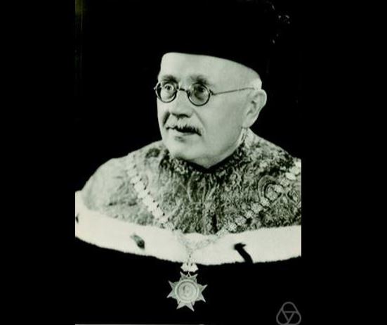
Remembering an Austrian mathematician Johann Radon (1887–1956) died on 25 May, in Vienna 🇦🇹, 65 years ago. 💐
#Radontransform #calculusofvariations #ラドン変換
👨🏫@zbMATH bit.ly/2QSTBv8
📷Johann Radon ©MFO
3
6

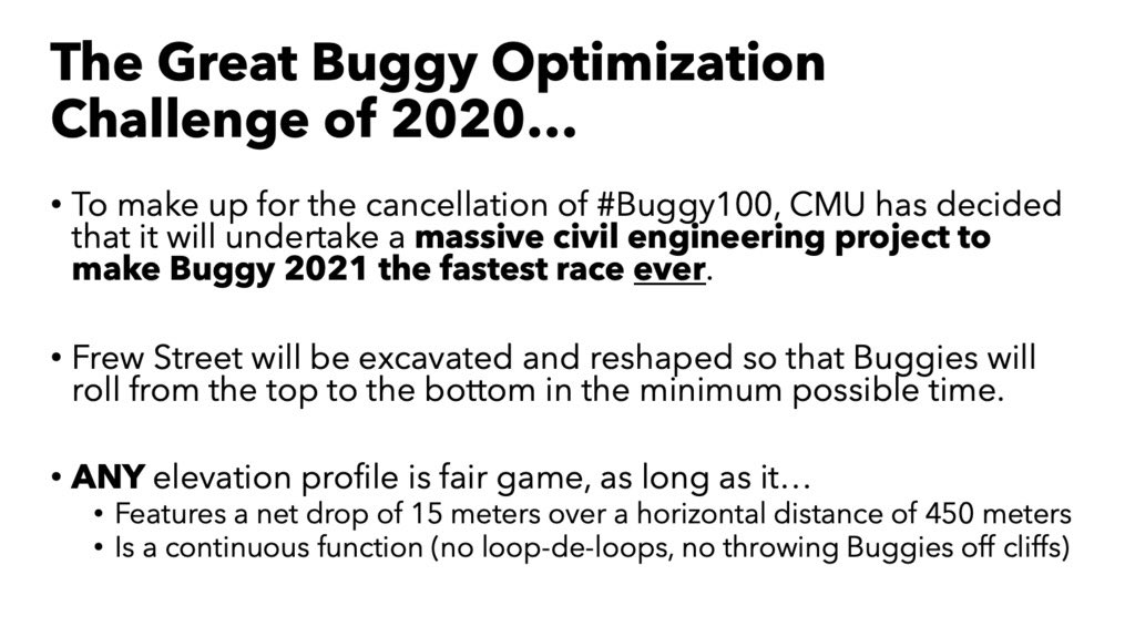
17 Apr 2020
To celebrate what would’ve been (my first!) #CMUCarnival @CarnegieMellon, @CMU_CEE 12-271 class today put forth a bold vision for #Buggy100: Reshaping Frew St for fastest possible race times. #Optimization #Sweepstakes #CalculusOfVariations #ThisIsCMU #Bug-chistochronesForTheWin


1
3
17

13 Mar 2018
Today in #PHY471: The brachistochrone problem is to find the path that causes a roller coaster to reach the end of its track in the shortest time. The path is a cycloid, animated below, but inverted. #calculusofvariations
1
2