Key takeaways from Phil Wong, Head of Capital Markets at SenseTime, during @HSBC‘s Private Bank Roundtable: China's #AI advantage today is increasingly defined by 𝗰𝗼𝘀𝘁, but also 𝗾𝘂𝗮𝗹𝗶𝘁𝘆 𝗼𝗳 𝗽𝗿𝗼𝗱𝘂𝗰𝘁, and in turn the ability to 𝗯𝗼𝗼𝘀𝘁 𝗽𝗿𝗼𝗱𝘂𝗰𝘁𝗶𝘃𝗶𝘁𝘆 and 𝗲𝗻𝗵𝗮𝗻𝗰𝗲 𝗲𝗳𝗳𝗶𝗰𝗶𝗲𝗻𝗰𝘆 for the end client, in order to maximise and optimise economic outcomes for end users. The real differentiator lies in 𝗰𝗿𝗲𝗮𝘁𝗶𝗻𝗴 𝗺𝗲𝗮𝘀𝘂𝗿𝗮𝗯𝗹𝗲 𝗯𝘂𝘀𝗶𝗻𝗲𝘀𝘀 𝗼𝘂𝘁𝗰𝗼𝗺𝗲𝘀 𝗮𝘁 𝘀𝗰𝗮𝗹𝗲, in addition to just a cost-benefit. How SenseTime is putting this into practice: • MultimodalＭodel #SenseNova U1 delivers strong performance with a smaller model footprint. • AI tools are streamlining daily workflows—such as data analysis and PPT generation with Office #Raccoon, and video production powered by #Seko. • AI infrastructure, #SenseCore, leverages compute-power co-optimization to reduce energy consumption and improve efficiency. Beyond these, keep an eye on spatial intelligence, world models, and other emerging AI frontiers.

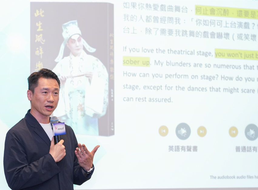
Through 𝗣𝘂𝗯𝗹𝗶𝘀𝗵𝗶𝗻𝗴 𝟯.𝟬 , we have applied our #MultimodalModel to help publishers in Hong Kong and the Chinese Mainland transform content into multilingual #eBooks and #audiobooks. This initiative supports publishers in reaching international markets and unlocks new opportunities for #IP commercialization. At a recent Sharing Session, Lewis Fung, Managing Director of SenseTime Hong Kong and Macau, outlined how we have leveraged #AI over the past year to streamline publishing workflows and improve #translation quality. He noted: “SenseTime is proud to support Publishing 3.0 , which helps Hong Kong connect #culture, #technology, and global markets, strengthening its role as an international hub for IP trading and cultural exchange.” Hong Kong is home to SenseTime’s headquarters and its key R&D centre. We are committed to leveraging its internationalization advantages to empower industries to thrive.

🚨 Call for Papers – CVPR 2026 "World Models" Workshop @CVPR We are excited to announce the Call for Papers for our CVPR 2026 Workshop on "🌍World Models Meet Active Sensing and Closed-Loop Planning". 🔗 beckschen.github.io/cvpr26wm… 📍 Location: CVPR 2026, Denver, USA 📅 June 3-4, 2026 This workshop aims to bring together researchers from computer vision, robotics, and embodied AI to explore new frontiers in world modeling. Invited Speakers: @YAloimonos @chelseabfinn C. Karen Liu, Jitendra Malik, @NickRoy_MIT 📌 Topics include (but are not limited to): • World Models • Active Sensing • Embodied Planning • Robotics ✨Lambda @LambdaAPI will sponsor the awards, including one Best Paper Award ($3,000 in compute credits), two Runner-Up Awards ($1,500 in compute credits each), and $400 in compute credits for each accepted paper. Powered by an amazing organizing team💥 @jieneng_chen @tianminshu @du_yilun Sanjeev Khudanpur, Cheng Peng, Rama Chellappa, @_Chen_Wei_ , Alan Yuille #CVPR2026 #WorldModel #ClosedLoopPlanning #Agents #EmbodiedAI #Robotics #ActiveSensing #VLA #MultimodalModel

If you're at #WACV2026, come visit our CVP poster! 📄 arxiv.org/pdf/2512.08135 [Poster session] 🗓️Sun, Mar 8, 2026 • 4:00 PM – 5:45 PM MST 📍Tucson Ballroom & Prefunction Space 84 Our authors will be there and are happy to chat about spatial reasoning, multimodal models, and vision-inspired architectures. 👋 @wacv_official @mlpcucsd @LambdaAPI #spatialReasoning #MultimodalModel #VLM #3dvision

🚀 Excited to share our #WACV2026 paper for 3D spatial reasoning: CVP: Central-Peripheral Vision-Inspired Multimodal Model for Spatial Reasoning Inspired by human vision, we introduce CVP, which combines: 👁️Target-affinity tokens (central vision) to focus on relevant objects 🌍Allocentric grids (peripheral vision) to capture global scene context This simple idea significantly improves 3D spatial reasoning, achieving SOTA performance across multiple benchmarks. 📄Paper: arxiv.org/pdf/2512.08135 🌐Page: zeyuan-chen.com/cvp/ #spatialReasoning #MultimodalModel #VLM @LambdaAPI @UCSD @mlpcucsd @wacv_official

エンタメから料理、受付、接客までこなす 汎用二足歩行人型ロボット youtu.be/9dvygD4G93c #bipedal #humanoid #robot #GeneralPurposeRobot #DeepReinforcementLearning #ImitationLearning #VLM #MultimodalModel #AgiBot

🚀 Step 3 is now open source! @StepFun_ai officially releases its next-gen multimodal reasoning model to the world - with major breakthroughs in performance and efficiency. 💬How the tech community is reacting? Check out the discussion on Zhihu: zhihu.com/question/193239477… 💡Co-founder Yibo Zhu also shared an in-depth breakdown of the system design before: zhuanlan.zhihu.com/p/1932920… #Step3 #OpenSource #MultimodalModel

人間と自然なやり取りができる二足歩行人型ロボット 自転車やホバーボードに乗ることもできる youtu.be/iyCjevFGLiA #bipedal #humanoid #robot #GeneralPurposeRobot #DeepReinforcementLearning #ImitationLearning #VLM #MultimodalModel #AgiBot #LingxiX2

When moving from just producing and transcoding video (and other modalities) into training a model, you need a well-defined data layout, a preprocessing pipeline, and a training loop that efficiently streams data through the GPU without excessive memory transfers. Below is a conceptual, end-to-end approach that integrates all these concepts: 1. Data Organization and Labeling A common approach for supervised training is to organize your dataset into a directory structure that encodes labels in folder names. Assume you have a dataset directory with train, val, and test splits, and each split contains subdirectories for each class label. Since you have multiple modalities (camera video, sound, LiDAR, radar, and even unknown sensors), store them in a systematic manner per sample: dataset/ train/ classA/ sample_000/ video.mp4 audio.wav lidar.bin radar.bin sensorX.data sample_001/ video.mp4 audio.wav lidar.bin radar.bin sensorX.data ... classB/ ... val/ ... test/ ... Rationale: Each sample’s modalities are grouped together in a single folder. Class labels come from the parent folder (e.g., classA). You can add a metadata file (e.g., metadata.json) to store timestamps, frame rates, or calibration data for LiDAR/radar if needed. 2. Preprocessing and Synchronization Before training, data often needs preprocessing. You might need to: Decode and preprocess video frames using FFmpeg with GPU acceleration. Extract or transform audio into spectrograms. Convert LiDAR point clouds into a structured tensor (like a voxel grid, or a depth/image-like representation). Represent radar data similarly (e.g., heatmap or text-based messages turned into a small image or embedding). GPU Memory and Data Transfers: To minimize CPU-GPU round trips, consider these steps: Video Preprocessing: Use a GPU-accelerated FFmpeg command: ffmpeg -hwaccel cuda -hwaccel_output_format cuda -i input_video.mp4 \ -vf "hwupload_cuda,scale_cuda=640:480:format=yuv420p" \ -c:v rawvideo -f rawvideo pipe:1 This outputs preprocessed frames directly from the GPU pipeline. If you must store them for training, you might hwdownload at the final step, but ideally keep them in a GPU-friendly compressed format (like a smaller-size H.264 or a sequence of images in NV12 format). Audio to GPU: Audio doesn’t decode to GPU memory as easily since it’s not GPU-accelerated by default. Convert audio to a log-mel spectrogram or another feature offline. Store it as a numpy .npy file (CPU memory). During training, you can load and optionally upload it to GPU. LiDAR/Radar/Unknown Sensors: Convert these sensor modalities into 2D/3D tensors. For example, LiDAR point clouds can be rasterized into a bird’s-eye-view image. Radar data can be turned into a range-Doppler map image. Perform these conversions offline or on-the-fly during training with efficient CPU/GPU augmentation libraries. If these are large, consider tiling or streaming them in smaller chunks and reassemble only what’s needed. 3. Dataset Preparation for Training Once the preprocessing is done, you might have: Compressed or frame-extracted video data stored in a GPU-friendly codec or as pre-processed tensors on disk. Audio spectrograms stored as .npy arrays. LiDAR and radar processed into image-like tensors or .npy arrays. Unknown sensors also converted to a known tensor format. Now you have a consistent set of input tensors per sample. A typical training input pipeline might look like this (in Python/PyTorch, as an example): class MultiModalDataset(torch.utils.data.Dataset): def __init__(self, root_dir, split='train', transform=None): # Index all samples and their modalities self.samples = self._load_samples(root_dir, split) self.transform = transform def _load_samples(self, root_dir, split): # Traverse `root_dir/split/classX/` and index all samples # Return a list of tuples: (video_path, audio_path, lidar_path, radar_path, label) pass def __getitem__(self, idx): sample = self.samples[idx] # Load each modality: video_tensor = self._load_video(sample['video_path']) # Possibly a GPU-decoding step if integrated audio_tensor = np.load(sample['audio_npy']) # CPU load, then torch.tensor() lidar_tensor = np.load(sample['lidar_npy']) radar_tensor = np.load(sample['radar_npy']) sensorX_tensor = np.load(sample['sensorX_npy']) # Convert to torch tensors audio_tensor = torch.from_numpy(audio_tensor) lidar_tensor = torch.from_numpy(lidar_tensor) radar_tensor = torch.from_numpy(radar_tensor) sensorX_tensor = torch.from_numpy(sensorX_tensor) # If transform, apply here (normalize, augment) if self.transform: # apply any data augmentations pass label = sample['label'] return (video_tensor, audio_tensor, lidar_tensor, radar_tensor, sensorX_tensor), label def __len__(self): return len(self.samples) Memory Considerations: If the video is stored in a GPU-friendly compressed format, you might integrate custom code that uses the FFmpeg libraries to decode frames directly to GPU memory, returning a GPU tensor. This avoids CPU-GPU copies. If that’s too complicated, just decode on CPU and tensor.to(device) once per batch. For large modalities, consider partial loading or streaming (e.g., only load the LiDAR segment you need per batch). Tiling large inputs into patches and processing them asynchronously can help. 4. Training Loop with Optimized Memory Usage During training: Use a DataLoader with num_workers>0 to parallelize data loading on the CPU side. Use pinned (page-locked) memory for DataLoader if available (pin_memory=True in PyTorch) to speed CPU-to-GPU transfers. Preallocate GPU tensors if your shapes are fixed, to reduce re-allocation costs each iteration. If using large frames or high-resolution, consider downscaling or partial processing as part of the transform pipeline. Example Training Command (Pseudocode): dataset = MultiModalDataset(root_dir='dataset', split='train', transform=some_transform) dataloader = torch.utils.data.DataLoader(dataset, batch_size=8, shuffle=True, num_workers=4, pin_memory=True) model = MultiModalModel() # A model that takes video audio lidar radar sensorX model.to('cuda') optimizer = torch.optim.Adam(model.parameters()) criterion = torch.nn.CrossEntropyLoss() for epoch in range(num_epochs): model.train() for (video, audio, lidar, radar, sensorX), label in dataloader: # Move to GPU video = video.to('cuda', non_blocking=True) audio = audio.to('cuda', non_blocking=True) lidar = lidar.to('cuda', non_blocking=True) radar = radar.to('cuda', non_blocking=True) sensorX = sensorX.to('cuda', non_blocking=True) label = label.to('cuda', non_blocking=True) optimizer.zero_grad() output = model(video, audio, lidar, radar, sensorX) loss = criterion(output, label) loss.backward() optimizer.step() 5. Integrating GPU-Accelerated Transcoding with Training If you need on-the-fly transcoding or augmentation at training time (e.g., random resizing or cropping video on the GPU), you can: Use FFmpeg’s GPU pipeline and a named pipe or shared memory. Your __getitem__ might call a function that runs an FFmpeg command line (or uses libav libraries) to decode a portion of the video directly into GPU memory. This would be more complex but can be done by writing custom C code or a Python extension that interfaces with the FFmpeg and CUDA APIs directly. The key is to keep data on GPU as long as possible, applying filters and scaling before handing the frames to PyTorch. 6. Handling Unknown Problem Gradients You mentioned being memory inefficient to optimize against an unknown problem gradient. This might mean experimenting with different input sizes, modalities, or GPU tiling strategies: Try first a straightforward approach (decode on CPU, transfer to GPU) and measure performance. If performance is insufficient, implement tiling: break large inputs into smaller chunks, process them asynchronously, and measure again. Adjust batch sizes, resolution, or tile sizes dynamically. Because the problem gradient is unknown, implement flexible code that can quickly switch between these strategies. 7. Summary A standardized folder structure: split/class/sample/ with multiple modalities per sample. Preprocess all modalities offline into formats that are easy to load during training (e.g., .npy for non-video, GPU-compatible videos). Use FFmpeg with GPU acceleration for video transformations before or during training. Implement a training dataset and DataLoader that can handle multiple modalities efficiently. Use pinned memory, asynchronous transfers, tiling, and GPU-friendly formats to reduce CPU-GPU bottlenecks. Continuously profile and adjust pipeline to handle unknown performance issues. This integrated approach moves from raw multimodal data on disk, through GPU-accelerated preprocessing with FFmpeg, into a training loop that minimizes memory transfers and can adapt to complex, unknown bottlenecks by adjusting strategies like tiling and streaming. Below is a more concrete, integrated scenario combining training, multiple modalities (video and others), and maintaining control via a running producer pipeline that provides data through shared memory or pipes. The goal is to create a setup where you can train a model directly on streaming data from a producer process, while also having static datasets on disk. This lets you adaptively control what frames, modalities, or segments you feed into the training loop in real-time. Key Points: 1. Producer-Consumer Setup Using Shared Memory or Named Pipes: We previously described using named pipes or shared memory (via shm_open, mmap) to pass decoded frames or preprocessed data from a producer to a consumer. Now we integrate that into the training loop: The producer (an FFmpeg-based pipeline, plus possibly custom code) runs continuously, decoding live video and converting LiDAR, radar, and unknown sensor data into a standardized tensor form. This producer writes data into a shared memory region or pipe. The training process (consumer) reads from this shared memory or pipe to get fresh training samples. By doing so, you have real-time control: you can send commands to the producer to change filters, modalities, or subsets of the data on the fly, and the training loop will adapt to whatever data comes through. 2. Hybrid Approach: Disk Live Feed: Your dataset may have a standard directory structure for historical data, as outlined before. You can load from disk for the bulk of your training samples. Additionally, insert a special “live” modality or sample entry that reads from the producer in memory. This gives you a hybrid scenario: Most samples: static data from disk (preprocessed .npy, .mp4, etc.) Some samples: live data from the producer pipeline (video frames, sensor arrays) read directly from shared memory. 3. Shared Memory Data Flow: The producer uses FFmpeg with GPU acceleration to decode and process frames. After processing (e.g., scaling video, converting LiDAR to an image, etc.), it writes the final tensors to a shared memory region. This shared memory can contain a header that indicates the shape, modality types, and a frame counter. Another region might store raw pixel or floating-point data. Semaphores or atomic flags signal when a new frame is ready. The training process waits on a semaphore from the producer indicating a new sample is ready, then reads the data, converts it to a tensor, and feeds it into the training loop. 4. Code Sketch (Conceptual, Not Full Production Code): Producer Side (C/C ): // Pseudocode: producer writes a single multimodal sample (video frame sensor arrays) to shared memory. // This can be integrated with FFmpeg’s decoding pipeline as shown before. struct sample_header { int frame_number; int video_width; int video_height; int video_channels; // e.g. 3 for RGB int lidar_width, lidar_height; // if representing LiDAR as image int radar_size; // arbitrary int sensorX_size; // arbitrary // possibly more fields... }; // Assume we have mapped shared memory region and semaphores as previously described. // After decoding and preparing a frame, and other modalities: sample_header *hdr = (sample_header *)shared_mem_base; unsigned char *data_ptr = (unsigned char*)(hdr 1); // Fill hdr with metadata hdr->frame_number = current_frame_number; hdr->video_width = 640; hdr->video_height = 480; hdr->video_channels = 3; hdr->lidar_width = 200; hdr->lidar_height = 200; hdr->radar_size = 1024; hdr->sensorX_size = 512; // Copy video frame data (e.g. 640*480*3 bytes) into data_ptr memcpy(data_ptr, video_frame_data, 640*480*3); data_ptr = 640*480*3; // Copy LiDAR data memcpy(data_ptr, lidar_image_data, 200*200); data_ptr = 200*200; // Copy radar data memcpy(data_ptr, radar_data, 1024); data_ptr = 1024; // Copy sensorX data memcpy(data_ptr, sensorX_data, 512); // Signal to consumer that a new sample is ready: sem_post(producer_sem); Consumer (Training) Side (Python with PyTorch): import torch import numpy as np import mmap import os from torch.utils.data import Dataset, DataLoader class LiveMultimodalDataset(Dataset): def __init__(self, disk_root, live_shared_mem_path, use_live_feed=True): self.disk_samples = self._index_disk(disk_root) self.use_live_feed = use_live_feed # Map shared memory self.mem_fd = os.open(live_shared_mem_path, os.O_RDWR) # Suppose we know total_size from configuration total_size = 640*480*3 200*200 1024 512 1024 # just example self.mmap_obj = mmap.mmap(self.mem_fd, total_size sizeof_header, mmap.MAP_SHARED, mmap.PROT_READ|mmap.PROT_WRITE) # Semaphores or signals handled externally, we assume a function wait_for_sample_ready() def _index_disk(self, root): # scan folder structure and return list of static samples samples = [] # ... return samples def __len__(self): return len(self.disk_samples) (1 if self.use_live_feed else 0) def __getitem__(self, idx): if self.use_live_feed and idx == len(self.disk_samples): # read from live feed self.wait_for_sample_ready() # wait on a semaphore or event from producer hdr = self._read_header() data = self._read_data(hdr) # Convert data to tensors video_tensor = torch.from_numpy(data['video']).float() lidar_tensor = torch.from_numpy(data['lidar']).float() radar_tensor = torch.from_numpy(data['radar']).float() sensorX_tensor = torch.from_numpy(data['sensorX']).float() # Example label: might come from an external source or a default label label = 0 return (video_tensor, lidar_tensor, radar_tensor, sensorX_tensor), label else: # load from disk sample = self.disk_samples[idx] # load static npy or mp4 data similarly # ... return (video_tensor, lidar_tensor, radar_tensor, sensorX_tensor), label def _read_header(self): self.mmap_obj.seek(0) # read sample_header fields (assume binary struct) # parse frame_number, sizes... # return a dict or object with metadata pass def _read_data(self, hdr): # read data arrays from shared memory according to hdr sizes self.mmap_obj.seek(sizeof_header) video_size = hdr.video_width * hdr.video_height * hdr.video_channels video_data = np.frombuffer(self.mmap_obj.read(video_size), dtype=np.uint8).reshape(hdr.video_height, hdr.video_width, hdr.video_channels) lidar_size = hdr.lidar_width * hdr.lidar_height lidar_data = np.frombuffer(self.mmap_obj.read(lidar_size), dtype=np.uint8).reshape(hdr.lidar_height, hdr.lidar_width) radar_data = np.frombuffer(self.mmap_obj.read(hdr.radar_size), dtype=np.uint8) sensorX_data = np.frombuffer(self.mmap_obj.read(hdr.sensorX_size), dtype=np.uint8) return {'video': video_data, 'lidar': lidar_data, 'radar': radar_data, 'sensorX': sensorX_data} def wait_for_sample_ready(self): # block until producer_sem signals a new sample pass # Now, training code: dataset = LiveMultimodalDataset(disk_root='dataset', live_shared_mem_path='/dev/shm/myshared', use_live_feed=True) dataloader = DataLoader(dataset, batch_size=4, shuffle=True) model = MultiModalModel() # hypothetical model model.cuda() optimizer = torch.optim.Adam(model.parameters()) criterion = torch.nn.CrossEntropyLoss() for epoch in range(10): for (video, lidar, radar, sensorX), label in dataloader: video = video.cuda(non_blocking=True) lidar = lidar.cuda(non_blocking=True) radar = radar.cuda(non_blocking=True) sensorX = sensorX.cuda(non_blocking=True) label = label.cuda(non_blocking=True) optimizer.zero_grad() output = model(video, lidar, radar, sensorX) loss = criterion(output, label) loss.backward() optimizer.step() 5. Dynamic Control Over the Producer: The producer can listen to commands (through another pipe or shared memory) and change what it’s writing. For example: Command: “Switch video to grayscale” Command: “Use LiDAR from a different sensor” Command: “Change radar processing method” The producer applies these changes, and the training loop automatically sees the different data in subsequent samples. This gives you end-to-end control: Start producer with FFmpeg custom code to decode and process all modalities in GPU memory, then write to shared memory. Producer can be commanded at runtime to alter filters or select different time segments of video. The training process continuously reads from both disk (for stable reference data) and from the live producer feed (for dynamic, real-time data) and trains the model. 6. Managing GPU vs CPU Memory Transfers: If you decode and preprocess on the GPU, you may still need to hwdownload to CPU for shared memory writing, since shared memory is accessible by CPU. If efficiency is paramount, consider using CUDA-IPC or GPU-aware shared memory (complex and platform-specific). Another approach: produce and consume entirely on the GPU if possible. Use CUDA inter-process communication (IPC) to share GPU memory buffers between producer and consumer processes. This is advanced and not directly supported by FFmpeg CLI, so you might implement custom code linking libav* libraries with CUDA IPC. For simplicity, the above code sticks to CPU shared memory. You can tile data or compress it before writing to reduce overhead. If frames are huge, tile them into chunks and process incrementally. Conclusion: This refined approach incorporates training directly on live pipeline data along with static datasets, gives you runtime control over the input via producer commands, and integrates multiple modalities. The final design involves: A producer process that decodes, processes, and places data into shared memory. A consumer (training) process that reads from both static disk-based datasets and the live shared memory feed. Control channels to send commands to the producer, altering the data that appears in the training loop. The ability to adapt strategies for memory handling, such as partial tiling or CUDA IPC, if needed.

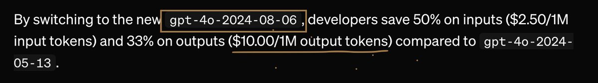
Big News! 🚀 @OpenAI releases GPT-4o, a multimodal model that's 50% cheaper for input tokens & 33% cheaper for output tokens! 💸 More affordable AI for developers! 🤖 #OpenAI #GPT4o #MultimodalModel #AIforAll @sama @OpenAIDevs

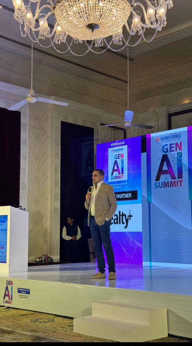
Demonstrating the use cases of Ask QX at BW Businessworld Gen AI Summit 2024 was an honor. I spoke about Ask QX’s ability to understand over 100 languages, real-time translation and effortless solutions in the text-to-text sphere. As we move ahead, QX Lab AI intends to launch its Multimodal model in May which can process data from multiple sources and provide more detailed and nuanced output. Our use case partnerships are another important area of focus. In the future, Ask QX will shape the evolution of Gen AI with an emphasis on collaboration, innovation and empowerment. @BWBusinessworld @QXLabAI #GenAISummit #BWBusinessworld #AskQX #MultimodalModel #Innovation #NextGenAI #AskQXLabAI #InnovativeTechnology #DigitalTransformation #GenerativeAI #BharatKaAI

🚀 Exciting news from Apple! Introducing MM1, a cutting-edge multimodal model for text and image data. By combining powerful architecture, diverse data sources, and innovative training techniques, MM1 sets new standards in multimodal AI research. #Apple #MM1 #AI #MultimodalModel

From #LargeLanguageModel to #MultimodalModel. Don't miss out on the technological advances of the past few years! Something amazing could happen.#AGI #ASI

From #LargeLanguageModel to #MultimodalModel. Don't miss out on the technological advances of the past few years! Something amazing could happen.#AGI #ASI

Don't miss out on the speed of evolution. #NFT #AGI #ASI #Multimodalmodel #blockchain

Explore Gemini, Google's versatile multimodal model available via Vertex AI! Developed by Google DeepMind, this model comprehends diverse inputs, merges different information types, and generates various outputs. In Vertex AI, prompt Gemini across text, video, code, audio, and images. Leverage Gemini's advanced reasoning and state-of-the-art generation capabilities to extract text from images, convert image text to JSON, and generate insightful answers from uploaded images for cutting-edge AI applications. Access over 130 generative AI models and tools! Key features include effortless model tuning, prompt-driven experimentation, Foundation Models, and APIs that connect models to real-world data and actions. Ready to explore the potential? Contact Comerit AI Services to learn more about Vertex AI and Gemini today! #VertexAI #GoogleGemini #AIInnovation #MultimodalModel #ComeritAIServices

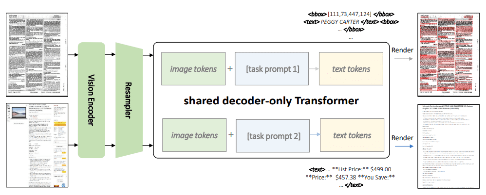
Kosmos-2.5: Pioneering Multimodal Literacy for Text-Intensive Images #AI #artificialintelligence #documentelementspositioning #fewshotlearning #languagedecoder #llm #machinelearning #markdowntextoutput #Media #Multimodalmodel #resamplermodule multiplatform.ai/kosmos-2-5-…

🤖🌐 Meet the future of robotics: PaLM-E! This groundbreaking embodied language model integrates real-world sensor data with language, enabling complex tasks and cross-modal understanding. From robotic manipulation to visual Q&A! 🔧🧠 #Robotics #AI #PaLM_E #MultimodalModel 🎥👇

Check out the new open-source multimodal AI model, "INTERN 2.5", by #SenseTime! Discover how it is revolutionizing image description, visual question-answering, visual reasoning, and text recognition. 👉sensetime.com/en/news-detail… #AI #multimodalmodel

Experience a New Level of AI Technology with GPT-4. The Next Generation of AI Technology: GPT-4 Takes the Lead. linkedin.com/feed/update/urn… #AI #GPT4 #AIrevolution #multimodalmodel #ArtificialIntelligence #MachineLearning #Technology #Innovation #Revolutionary #NewLevel