
Apr 14
Quantum Mechanics Series Lecture 4
Lecture 1 established that ρ(x,t) = |ψ(x,t)|² behaves like a conserved probability density.
Lecture 2 showed what drives that flow. We also saw that writing ψ = r exp(iθ) makes the probability current proportional to the phase gradient, making it clear that phase geometry literally steers the motion.
Lecture 3 then showed that the centroid of that flow can move almost classically when the packet is tight and the external potential is smooth.
However, that raises yet another question. If the centroid can look classical, why does the full wave still spread, bend, split, and interfere in ways no classical particle cloud would?
This is because the wave is not driven only by the external potential. It is also driven by its own curvature.
Write
ψ(x,t) = r(x,t) exp(iθ(x,t))
with ρ = r². Then Schrödinger’s equation gives two coupled real equations. One is the continuity equation you already know. The other looks like a Hamilton-Jacobi equation, but with one extra term:
Q = −(1/2m) ∇²r / r
This is the so-called Quantum Potential. It depends entirely on how the amplitude bends across space. So, the wave is being shaped not only by V(x,t), but also by the geometry of its own envelope.
In the animation, the upper surface is still |ψ| and its skin is still colored by arg(ψ). The glowing threads still trace the probability current. But now a second membrane hangs underneath. That lower membrane encodes the quantum potential Q itself. The porcelain bead marks the quantum centroid. The amber bead follows a classical centroid under the same external V. When those paths separate, the lower membrane tells you why. The difference is not magic but the extra term classical mechanics does not have.
The math breakdown:
Start from Schrödinger evolution in units with ħ = 1:
i ∂ψ/∂t = [ −(1/2m) ∇² V(x,t) ] ψ
Write the state in polar form:
ψ = r exp(iθ)
Then
ρ = |ψ|² = r²
From the imaginary part, you recover probability conservation:
∂ρ/∂t ∇·j = 0
with
j = (1/m) Im(ψ* ∇ψ) = (ρ/m) ∇θ
So the local velocity field is
v = j / ρ = ∇θ / m
Now take the real part of Schrödinger’s equation. That gives
∂θ/∂t |∇θ|² / (2m) V Q = 0
where
Q = −(1/2m) ∇²r / r
This is the classical Hamilton-Jacobi equation with one extra term. That extra term is what makes quantum motion locally different from classical motion.
Take a gradient of that phase equation and use v = ∇θ / m. Then the flow obeys an Euler-like equation:
∂v/∂t (v·∇)v = −(1/m) ∇(V Q)
In other words, there are really two forces in the problem. One comes from the external potential V. The other comes from the wave’s own curvature through Q.
That is why Ehrenfest is only approximate. The centroid can still satisfy
d⟨x⟩/dt = ⟨p⟩/m
d⟨p⟩/dt = −⟨∇V⟩
but the internal shape of the packet evolves under the combined influence of V and Q. When the packet stays broad and smooth, Q is gentle and the motion looks more classical. When the packet develops sharp curvature or interference structure, Q becomes strong and the classical picture breaks down.
That is what this scene is designed to show live.
#QuantumMechanics #Wavefunction #SchrodingerEquation #BornRule #ProbabilityCurrent #ContinuityEquation #Phase #EhrenfestTheorem #QuantumPotential #Madelung #HamiltonJacobi #MathematicalPhysics #Mathematics #Physics
11
88
519
20,408
Apr 14
Quantum Mechanics Series Lecture 3
Lecture 1 earned the right to call ρ(x,t) = |ψ(x,t)|² a probability density by showing that Schrödinger evolution forces a continuity equation, ∂ρ/∂t ∇·j = 0. Lecture 2 then answered the next question:
What actually steers that flow?
Writing ψ = r exp(iθ) turns the current into density times phase gradient. So, phase geometry literally drives the streamlines. Quantized vortices appear where that phase winds in discrete units.
Lecture 3 asks the next natural followup question
If probability flows, does the bulk of that flow have a trajectory?
Ehrenfest says yes. The centroid of the wavepacket can move almost classically when the packet is tight enough and the potential is smooth enough.
In this render, the surface height is |ψ(x,t)| and the surface skin is colored by arg(ψ(x,t)). The porcelain bead rides on the surface at the quantum centroid ⟨x⟩(t). The amber bead tracks a classical centroid evolved under the same V(x,t). The steel arrow points along ⟨p⟩. The glowing threads trace the probability current itself. It is still the same ψ from the earlier lectures. We are just pushing the same objects one step further and asking whether their collective motion begins to look classical.
The math breakdown:
We treat the state as a complex field ψ(x,t) on the plane, with x in R². The Born rule defines the probability density
ρ(x,t) = |ψ(x,t)|²
and Schrödinger evolution, in units with ħ = 1, is
i ∂ψ/∂t = [ −(1/2m) ∇² V(x,t) ] ψ
From Lecture 1 we already have the continuity equation
∂ρ/∂t ∇·j = 0
with probability current
j = (1/2mi) ( ψ* ∇ψ − ψ ∇ψ* )
= (1/m) Im(ψ* ∇ψ)
From Lecture 2, writing ψ = r exp(iθ) turns this into
j = (ρ/m) ∇θ
So now we ask another question. What happens to the centroid of that flowing density?
Define the position centroid and mean momentum by
⟨x⟩(t) = ∫ x ρ(x,t) dx
⟨p⟩(t) = ∫ ψ*(x,t) [ −i ∇ ] ψ(x,t) dx
Ehrenfest’s theorem states
d⟨x⟩/dt = ⟨p⟩/m
d⟨p⟩/dt = −⟨∇V(x,t)⟩
The first identity drops straight out of the continuity equation. So it really is built from the same probability-flow picture as the earlier lectures. Start from the centroid:
d⟨x⟩/dt
= ∫ x (∂ρ/∂t) dx
= −∫ x (∇·j) dx
Integrate by parts. The boundary term vanishes because the wavefunction decays at the edges. This leaves
−∫ x (∇·j) dx = ∫ j dx
Hence
d⟨x⟩/dt = ∫ j dx
Now substitute the expression for j:
∫ j dx
= (1/m) ∫ (1/2i)(ψ* ∇ψ − ψ ∇ψ*) dx
= (1/m) ∫ ψ*(−i ∇)ψ dx
= ⟨p⟩/m
So we get
d⟨x⟩/dt = ⟨p⟩/m
The second identity comes from differentiating ⟨p⟩, inserting Schrödinger’s equation for ∂ψ/∂t and ∂ψ*/∂t, and integrating by parts. The kinetic pieces cancel. The potential contributes the force term:
d⟨p⟩/dt = −⟨∇V⟩
Then comes the classical bridge. If the packet is narrow and the potential does not change much across it, the mean force is close to the force at the mean position:
⟨∇V⟩ ≈ ∇V(⟨x⟩)
so the centroid approximately obeys
m d²⟨x⟩/dt² ≈ −∇V(⟨x⟩)
That is the point of the animation. It takes the same ingredients from Lectures 1 and 2, namely ρ, j, and phase, and asks whether their collective motion begins to follow Newton’s law.
#QuantumMechanics #Wavefunction #SchrodingerEquation #BornRule #ProbabilityCurrent #ContinuityEquation #Phase #Vortices #EhrenfestTheorem #ExpectationValues #MathematicalPhysics #Mathematics #Physics
9
21
163
5,780
Apr 12
Quantum Mechanics Series Lecture 2
Lecture 1 gave us one of the cleanest facts in quantum mechanics
If ψ(x,t) is the state, then ρ(x,t) = |ψ(x,t)|² behaves like a probability density, and Schrödinger evolution makes that density satisfy a continuity equation.
So, if ρ flows like a fluid, then what determines the flow?
To answer that, write the wavefunction as
ψ(x,t) = r(x,t) exp(iθ(x,t)).
Now the picture sharpens. The magnitude r tells you how much probability is present at a point. The phase θ tells you how that probability is directed. But how exactly does phase enter the motion?
When you expand the current,
j = (1/m) Im(ψ* ∇ψ),
it reduces to
j = (ρ/m) ∇θ.
That is the key step. The current is driven by the phase gradient. So the flow lines are not decorative. They are the geometry of phase made visible.
Then another question appears. Can the phase wind around space in any arbitrary way?
The answer is no, because ψ has to come back to the same value after going around a closed loop, the total phase change cannot be arbitrary. It must be an integer multiple of 2π:
∮ ∇θ · dl = 2πn.
That is where quantized vortices come from. They are not features we bolt onto the theory. They are topological defects the mathematics allows only in discrete units.
In the 2D render reveals the underlying mechanism of probability current bending around isolated vortex charges.
The math breakdown:
We describe the state by a complex field ψ(x,t) on the plane, with x in R². The Born rule defines the probability density
ρ(x,t) = |ψ(x,t)|².
Schrödinger evolution, in units with ħ = 1, is
i ∂ψ/∂t = [ −(1/2m) ∇² V(x,t) ] ψ.
Why does this preserve probability?
Start from
ρ = ψ*ψ.
Differentiate:
∂ρ/∂t = ψ* (∂ψ/∂t) ψ (∂ψ*/∂t).
Now insert Schrödinger’s equation and its complex conjugate:
∂ψ/∂t = (1/i) [ −(1/2m) ∇²ψ Vψ ]
∂ψ*/∂t = (−1/i) [ −(1/2m) ∇²ψ* Vψ* ].
What survives after substitution?
The potential terms cancel. The rest rearranges into the continuity equation
∂ρ/∂t ∇·j = 0
with probability current
j = (1/2mi) ( ψ* ∇ψ − ψ ∇ψ* )
= (1/m) Im(ψ* ∇ψ).
So ρ really does behave like a conserved fluid density, and j is its flux.
But what actually steers that flux?
Write ψ in polar form:
ψ(x,t) = r(x,t) exp(iθ(x,t)).
Then
∇ψ = exp(iθ) (∇r i r ∇θ).
So
ψ* ∇ψ = r (∇r i r ∇θ).
Taking the imaginary part gives
Im(ψ* ∇ψ) = r² ∇θ = ρ ∇θ.
Hence
j = (ρ/m) ∇θ.
That is the central statement of this lecture:
The phase gradient sets the direction and speed of the flow, scaled by the density and the mass.
Now one last question. Why are the vortices quantized?
Because ψ must be single-valued. If you go once around a closed loop and return to the same point, the complex field must return to the same value. That forces the total phase winding to satisfy
∮ ∇θ · dl = 2πn, with n in Z.
The integer n is the vortex charge. At the vortex core, ρ is nearly zero, the phase becomes undefined, and the current circulates around that defect.
#QuantumMechanics #Wavefunction #SchrodingerEquation #BornRule #ProbabilityCurrent #ContinuityEquation #Phase #Vortices #TopologicalDefects #ComplexAnalysis #MathematicalPhysics #Mathematics #Physics
13
53
257
10,602

Mar 16
🚨 Crypto Update:
BTC Pump Potential to New ATH & XRP Price Targets Hey community! Pinning this for visibility as we navigate the volatile 2026 crypto market. Bitcoin (BTC) is showing signs of recovery after dipping to around $66K-$73K following its October 2025 all-time high (ATH) of approximately $122K-$125K.
With the market cooling off, let's break down the pump probability and what it means for XRP.BTC Pump Analysis & ATH ProbabilityCurrent Setup: BTC has rebounded slightly, trading above $93K in early 2026 signals, but it's still down ~47% from its peak.
Analysts see a "bullish trend" emerging, with potential for a breakout if it holds above key supports like $85K or the 200-day moving average.
Pump Probability to New ATH: High optimism for a rally—predictions range from $100K short-term (with a possible retrace to $57K-75K) to $125K by year-end.
Broader forecasts go as high as $225K if regulatory clarity and Fed liquidity boost sentiment.
However, some warn of a "nightmare scenario" crash if correlations with stocks falter.
Overall probability? I'd peg it at 60-70% for a new ATH in 2026, based on cycle patterns and recent consolidation—watch for a push to $107K-$112K if we avoid deep corrections.
XRP Price Targets if BTC Pumps to ATHCorrelation Factor: XRP often moves with BTC during pumps, especially in bull cycles. If BTC hits a new ATH (say $125K ), XRP could see amplified gains due to Ripple's partnerships, regulatory wins, and adoption in cross-border payments.
Conservative Targets: Base case: $2.50-$3.50 by mid-2026, assuming partial adoption and BTC momentum.
Bullish outlook: $5-$6 if catalysts like SEC clarity align.
Ambitious Projections: Viral predictions suggest $18.40 (a 794% surge from ~$1.54 current levels) if XRP market cap hits $1.84T, equating to 5,000 XRP per 1 BTC.
To reclaim its $3.84 historical ATH, four key catalysts needed: regulatory green lights, Bitcoin surge, institutional inflows, and tech upgrades.
Longer-term: $5.75 by 2030, but a BTC pump could accelerate to $4 if resistance at $1.55-$2 flips to support.
DYOR—markets are unpredictable, but with BTC's potential rebound, alts like XRP could shine.
Ok?
2
4
77
Feb 8
Watching Probability Flow in Quantum Mechanics
In the previous post we earned the right to call ρ(x,t) = |ψ(x,t)|² a probability density. Schrödinger evolution doesn’t just move ψ around. It forces a continuity equation
∂ρ/∂t ∇·j = 0
so probability really flows, with a current j.
The next step is seeing what actually steers that flow. Write ψ = r exp(iθ) and the current turns into
j = (ρ/m) ∇θ
So phase geometry isn’t decoration. It literally draws the streamlines. And once you see that, vortices stop looking mystical. They’re just places where the phase winds by ±2π around a low-density core.
After that, the natural question is hard to avoid. If probability flows, does the bulk of it move like something with a trajectory? Ehrenfest’s theorem says yes, in the regime where the packet is tight and the potential is smooth:
d⟨x⟩/dt = ⟨p⟩/m
d⟨p⟩/dt = −⟨∇V⟩
That’s what this animation is tying together.
In the 3D panel, the surface height is |ψ(x,t)| and the surface skin is colored by the phase arg ψ. The porcelain bead rides along the quantum centroid ⟨x⟩(t). The amber bead follows a classical centroid evolved under the same potential V(x,t). The teal arrow points along the mean momentum ⟨p⟩. Same environment, two notions of motion, tracked side by side.
In the 2D panel you’re seeing the same ψ, just from a different angle. Phase is still color, amplitude is still brightness, but now the current field shows up directly. The glowing ribbons are streamlines of j. The small charged defects are vortices, where the phase wraps by ±2π around a point where the density thins out. Nothing new has been added. It’s the same objects, just viewed through different lenses.
The math breakdown
We treat the state as a complex field ψ(x,t) on the plane. The Born rule gives the density
ρ(x,t) = |ψ(x,t)|²
Schrödinger evolution, in units with ħ = 1, is
i ∂ψ/∂t = [ −(1/2m) ∇² V(x,t) ] ψ
From the continuity equation,
∂ρ/∂t ∇·j = 0,
the probability current is
j = (1/2mi)(ψ* ∇ψ − ψ ∇ψ*)
= (1/m) Im(ψ* ∇ψ)
Writing ψ = r exp(iθ) makes the geometry explicit:
j = (ρ/m) ∇θ
Now define the centroid and mean momentum,
⟨x⟩(t) = ∫ x ρ(x,t) dx
⟨p⟩(t) = ∫ ψ*(x,t)[−i ∇]ψ(x,t) dx
The first Ehrenfest identity drops straight out of continuity. Differentiate ⟨x⟩ and integrate by parts:
d⟨x⟩/dt
= ∫ x (∂ρ/∂t) dx
= −∫ x (∇·j) dx
= ∫ j dx
= ⟨p⟩/m
So
d⟨x⟩/dt = ⟨p⟩/m
The second one comes from differentiating ⟨p⟩, using Schrödinger to replace ∂ψ/∂t and ∂ψ*/∂t, then integrating by parts so the kinetic contributions cancel and the potential contributes a force term:
d⟨p⟩/dt = −⟨∇V⟩
When the wavepacket is narrow and V is nearly linear across it,
⟨∇V⟩ ≈ ∇V(⟨x⟩)
and the centroid follows an almost-Newtonian law,
m d²⟨x⟩/dt² ≈ −∇V(⟨x⟩)
That’s the punchline. Density, current, phase, and centroid motion all hook together into one picture you can actually watch.
#QuantumMechanics #Wavefunction #SchrodingerEquation #BornRule #ProbabilityCurrent #ContinuityEquation #Phase #Vortices #EhrenfestTheorem #MathematicalPhysics
5
38
270
9,249
Jan 2
This is our last lecture on our Quantum Mechanics series.
We bow out with an application🫡
Electron holography is a fitting finale because it turns our whole lecture series into a single, concrete instrument. In our scene, we launch a coherent electron wave ψ across a TEM-style stage, force it to split and wrap around a flux-carrying nanoring in the middle, then recombine it downstream.
The detector doesn’t see phase directly, it only sees intensity ρ = |ψ|², so when we sweep the Aharonov-Bohm knob φ_AB(t) (implemented as a phase shift applied to the upper-arm corridor), the only possible outcome is that the interference cross-term changes and the hologram fringes on the detector plate slide. Geometry stays fixed, forces stay the same along the arms, and yet the picture moves, because it has to…it’s the algebra of squaring a sum made visible.
In the 3D scene, the surface height is |ψ(x,t)| and the surface skin is arg(ψ(x,t)). The metallic ring is the flux-carrying core the flow wraps around. The glowing filaments are streamlines of v = j/(ρ eps), built from j = (ħ/m) Im(ψ*∇ψ), so you’re literally watching the probability current split, bend, and recombine. The translucent plate above is the hologram detector: it displays the measured intensity |ψ|², and when the Aharonov–Bohm knob φ_AB(t) ramps, the fringe ridges slide smoothly even though the geometry is unchanged.
The math breakdown
We model the electron beam in the transverse plane x in R² with a complex wavefunction ψ(x,t). The measurable intensity is
ρ(x,t) = |ψ(x,t)|²
Schrödinger evolution is
i ħ ∂ψ/∂t = [ -(ħ²/2m) ∇² V(x) ] ψ
This implies probability conservation
∂ρ/∂t ∇·j = 0
with probability current
j = (ħ/2mi)( ψ* ∇ψ - ψ ∇ψ* )
= (ħ/m) Im(ψ* ∇ψ)
and the flow field used for streamlines is
v = j / (ρ eps)
Now the holography step is interference. Two coherent contributions reach the same detector pixel x:
ψ(x) = ψ₁(x) ψ₂(x)
So the measured intensity becomes
ρ(x) = |ψ(x)|²
= |ψ₁ ψ₂|²
= |ψ₁|² |ψ₂|² 2 Re(ψ₁ ψ₂*)
Write each contribution in polar form
ψ₁(x) = r₁(x) exp(i θ₁(x))
ψ₂(x) = r₂(x) exp(i θ₂(x))
Then
ψ₁ ψ₂* = r₁ r₂ exp(i(θ₁ − θ₂))
so the cross-term is
2 Re(ψ₁ ψ₂*) = 2 r₁ r₂ cos(θ₁(x) − θ₂(x))
That cosine is the fringe engine.
Now the Aharonov-Bohm phase is a phase-only shift produced by enclosed magnetic flux Φ. The relative phase shift is
φ_AB = (e/ħ) Φ
So we model it as
ψ₂(x) → ψ₂(x) exp(i φ_AB)
which updates the phase difference
(θ₁ − θ₂) → (θ₁ − θ₂) − φ_AB
and therefore the measured intensity becomes
ρ(x; φ_AB) = r₁² r₂² 2 r₁ r₂ cos( (θ₁ − θ₂) − φ_AB )
As φ_AB(t) is swept, the interference fringes translate continuously on the detector plane. Same amplitudes, same device geometry ...only phase changed.
#QuantumMechanics #Wavefunction #SchrodingerEquation #BornRule #ProbabilityCurrent #ContinuityEquation #Phase #Interference #AharonovBohm #ElectronHolography #TEM #MathematicalPhysics #Physics #Mathematics
9
55
306
12,902
Jan 2
Lecture 5 of our Quantum Mechanics series.
Lecture 2 taught us to treat ρ = |ψ|² as a real probability density because Schrödinger evolution forces a continuity equation, so probability doesn’t just appear on the screen, it moves. Lecture 3 showed what drives that motion...write ψ = r e^(iθ) and the current becomes j = (ρ/m) ∇θ, so phase geometry is literally the steering wheel, and vortices show up as quantized phase defects. Lecture 4 then connected that fluid picture to something your classical intuition recognizes: The centroid ⟨x⟩ can move almost Newton-like even while the full ψ stays spread out and wavy.
Lecture 5 is the next important question:
If probability is a conserved fluid with a velocity field, what is the real dynamical law for that velocity itself?
The answer is that Schrödinger hides a second equation...phase evolves like a Hamilton-Jacobi equation, but with one extra term that has no classical twin. That term is the so-called "quantum potential," and it is exactly where tunneling, diffraction, and interference forces come from. It’s not mysterious but a concrete correction in the phase equation that survives even when there is no classical force to push the flow.
In the animation, you’ll see the density surface and the current ribbons behave like a fluid, but you’ll also see moments where the flow bends and accelerates in places a classical particle wouldn’t. That’s the quantum potential acting as a pressure-like term sourced by curvature of r = |ψ|. Phase still steers (Lecture 3), probability still conserves (Lecture 2), and the centroid can still look classical (Lecture 4). Lecture 5 explains why all three can be true at once, and where the extra quantum behavior enters the dynamics.
The math breakdown
We start from the same objects as Lectures 2-4.
Born rule:
ρ(x,t) = |ψ(x,t)|²
Polar form:
ψ(x,t) = r(x,t) exp(i θ(x,t))
ρ = r²
Probability current (Lecture 2), with the phase mechanism (Lecture 3):
j = (1/2mi)(ψ∇ψ − ψ∇ψ)
j = (ρ/m) ∇θ
Define the local velocity field v by "current = density × velocity":
v(x,t) = j/ρ = (1/m) ∇θ
Now plug ψ = r e^(iθ) into Schrödinger’s equation
i ∂ψ/∂t = [ −(1/2m) ∇² V(x,t) ] ψ
and separate real and imaginary parts.
Imaginary part gives the continuity equation again:
∂ρ/∂t ∇·(ρ v) = 0
Real part gives the phase dynamics:
∂θ/∂t (1/2m) |∇θ|² V Q = 0
where the extra term is the quantum potential
Q(x,t) = − (1/2m) (∇²r)/r
= − (1/4m) [ ∇²ρ / ρ − (1/2) |∇ρ|² / ρ² ]
(That second form is the same thing written in ρ instead of r.)
Now differentiate the phase equation in space to get an Euler-like law for v.
Since v = (1/m)∇θ,
∂v/∂t (v·∇)v = −(1/m) ∇(V Q)
Compare to classical Hamilton–Jacobi. If Q were zero, this is exactly the classical force law for a fluid of trajectories driven by V. The single new ingredient is Q, which depends on curvature of r (equivalently ρ). That’s why interference can push the flow around even in regions where V is flat.
This also matches the Lecture 4 story when the packet is narrow and smooth. In that regime, Q is small across the bulk, and the centroid approximately follows Newton:
m d²⟨x⟩/dt² ≈ −∇V(⟨x⟩)
But when r develops sharp structure (nodes, fringes, vortices), Q becomes large and the flow does something decisively nonclassical.
#QuantumMechanics #Wavefunction #SchrodingerEquation #BornRule #ProbabilityCurrent #ContinuityEquation #Phase #Madelung #HamiltonJacobi #QuantumPotential #HydrodynamicFormulation #EhrenfestTheorem #MathematicalPhysics #Mathematics #Physic
8
38
194
7,659
Jan 2
Things are heating up 🔥
Lecture 4 of our Quantum Mechanics series.
Lecture 2 earned the right to call ρ(x,t) = |ψ(x,t)|² a probability density by showing Schrödinger evolution forces a continuity equation, ∂ρ/∂t ∇·j = 0. Lecture 3 then revealed what actually steers that flow...writing ψ = r exp(iθ) makes the current j become "density × phase-gradient," so phase geometry literally draws the streamlines and quantized vortices show up as phase winding defects.
Lecture 4 is the next link in that same chain...once you accept that probability flows, you can ask whether the bulk of that flowing density has a trajectory...and Ehrenfest says yes, its centroid moves almost classically when the packet is tight and the potential is smooth.
In the 3D panel, the surface height is |ψ(x,t)| and the surface skin is colored by arg(ψ(x,t)). The porcelain bead rides on the surface at the quantum centroid ⟨x⟩(t), the amber bead is a classical centroid integrated under the same V(x,t), and the teal arrow points along ⟨p⟩.
In the 2D panel, the background uses the same encoding (phase as color, amplitude as brightness), but now you can see the current field...the glowing ribbons are streamlines of j, and the small charged defects are vortices where the phase winds by ±2π around a low-density core. Both panels are the same ψ, just two ways of seeing the same objects from Lectures 2 and 3.
The math breakdown
We treat the state as a complex field ψ(x,t) on the plane (x in R²). The Born rule defines the probability density
ρ(x,t) = |ψ(x,t)|²
Schrödinger evolution (ħ = 1 units) is
i ∂ψ/∂t = [ −(1/2m) ∇² V(x,t) ] ψ
From Lecture 2 we have the continuity equation
∂ρ/∂t ∇·j = 0
with probability current
j = (1/2mi) ( ψ* ∇ψ − ψ ∇ψ* )
= (1/m) Im(ψ* ∇ψ)
From Lecture 3, writing ψ = r exp(iθ) turns that into
j = (ρ/m) ∇θ
Now define the centroid and mean momentum:
⟨x⟩(t) = ∫ x ρ(x,t) dx
⟨p⟩(t) = ∫ ψ*(x,t) [ −i ∇ ] ψ(x,t) dx
Ehrenfest’s theorem states
d⟨x⟩/dt = ⟨p⟩/m
d⟨p⟩/dt = −⟨∇V(x,t)⟩
Derive the first identity directly from the continuity equation (so it visibly depends on Lecture 2). Start from ⟨x⟩:
d⟨x⟩/dt
= ∫ x (∂ρ/∂t) dx
= −∫ x (∇·j) dx
Integrate by parts (boundary term vanishes because ρ → 0 at the edges):
−∫ x (∇·j) dx = ∫ j dx
So
d⟨x⟩/dt = ∫ j dx
Now substitute j and rewrite using Im(z) = (z − z*)/(2i):
∫ j dx
= (1/m) ∫ (1/2i)(ψ* ∇ψ − ψ ∇ψ*) dx
= (1/m) ∫ ψ*(−i ∇)ψ dx
= ⟨p⟩/m
Therefore
d⟨x⟩/dt = ⟨p⟩/m
The second identity comes from differentiating ⟨p⟩, using Schrödinger’s equation to replace ∂ψ/∂t and ∂ψ*/∂t, and integrating by parts so the kinetic contributions cancel while the potential contributes a force term:
d⟨p⟩/dt = −⟨∇V⟩
When V is nearly linear across the wavepacket (narrow packet, smooth potential), the mean force is approximately the force at the mean position:
⟨∇V⟩ ≈ ∇V(⟨x⟩)
and you get the Newton-like approximation
m d²⟨x⟩/dt² ≈ −∇V(⟨x⟩)
That’s what the animation is testing live using the same objects from Lectures 2 and 3...ρ, j, and phase.
#QuantumMechanics #Wavefunction #SchrodingerEquation #BornRule #ProbabilityCurrent #ContinuityEquation #Phase #Vortices #EhrenfestTheorem #ExpectationValues #MathematicalPhysics #Mathematics #Physics
5
41
224
8,350
Jan 1
Lecture 3 of our Quantum Mechanics series.
Lecture 2 gave us the one clean privilege quantum theory offers: treat ψ(x,t) as the state and ρ(x,t) = |ψ(x,t)|² as probability, because Schrödinger evolution forces ρ to obey a continuity equation. Lecture 3 is what that continuity equation is really telling you. If ρ behaves like a fluid, then the only question that matters is:
What is the velocity field?
Write
ψ(x,t) = r(x,t) exp(i θ(x,t)).
The magnitude r sets how much probability is sitting there. The phase θ sets where it tries to go. When you unpack the current j = Im(ψ* ∇ψ), it collapses to j = (ρ/m) ∇θ, which means the flow lines you draw are literally contours of phase geometry. Then the constraint that makes the picture bite: ψ has to be single-valued, so θ can’t wind by an arbitrary amount. Around any closed loop the total phase change must be 2π n, with n an integer. That’s why vortices aren’t features you add...they’re defects the math permits, in quantized units.
In the render you see both layers at once...the 3D surface shows |ψ| breathing while the phase skin slides, and the 2D panel exposes the engine...current lines steering around discrete vortex charges.
The math breakdown
We write the state as a complex field ψ(x,t) on the plane (x in R²). The Born rule defines the probability density
ρ(x,t) = |ψ(x,t)|²
Schrödinger evolution (ħ = 1 units) is
i ∂ψ/∂t = [ −(1/2m) ∇² V(x,t) ] ψ
Now derive conservation of probability. Start with ρ = ψ*ψ:
∂ρ/∂t = ψ* (∂ψ/∂t) ψ (∂ψ*/∂t)
Use Schrödinger and its complex conjugate:
∂ψ/∂t = (1/i) [ −(1/2m) ∇²ψ Vψ ]
∂ψ*/∂t = (−1/i) [ −(1/2m) ∇²ψ* Vψ* ]
Substitute. The V terms cancel, and the remaining terms rearrange into the continuity equation
∂ρ/∂t ∇·j = 0
with probability current
j = (1/2mi) ( ψ* ∇ψ − ψ ∇ψ* )
= (1/m) Im(ψ* ∇ψ)
So "probability density" really behaves like a conserved fluid density with flux j.
Now expose the phase mechanism. Write ψ in polar form
ψ(x,t) = r(x,t) exp(i θ(x,t))
Compute the gradient
∇ψ = exp(iθ) (∇r i r ∇θ)
Then
ψ* ∇ψ = r (∇r i r ∇θ)
Taking the imaginary part gives
Im(ψ* ∇ψ) = r² ∇θ = ρ ∇θ
So the current becomes
j = (ρ/m) ∇θ
That’s the steering-wheel statement:
Phase gradient sets the flow direction and speed (modulated by density and m).
Finally, quantized vortices.
Because ψ must be single-valued, going around any closed loop must return the same complex value. That forces the phase winding to be an integer multiple of 2π:
∮ ∇θ · dl = 2π n with n in Z
n is the vortex charge. Vortex cores sit where ρ ≈ 0 (phase is undefined), and the current streamlines circulate around them.
#QuantumMechanics #Wavefunction #SchrodingerEquation #BornRule #ProbabilityCurrent #ContinuityEquation #Phase #Vortices #TopologicalDefects #ComplexAnalysis #MathematicalPhysics #Mathematics #Physics
28
154
1,087
38,020

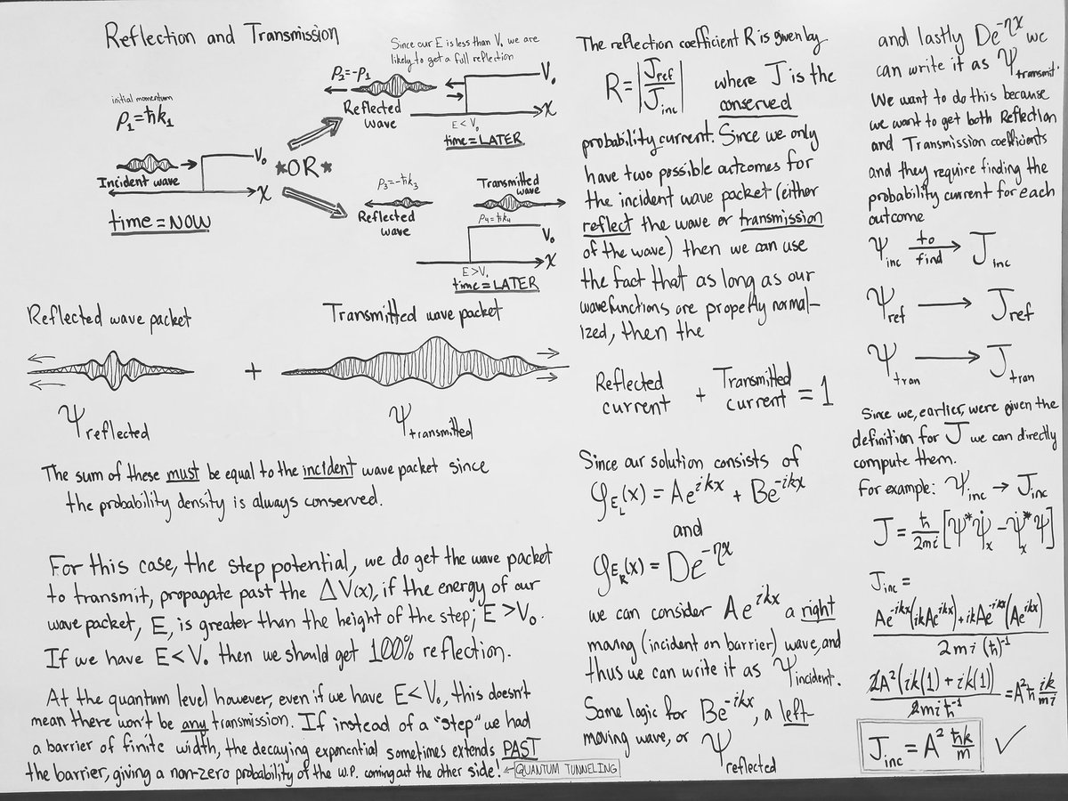
24 Mar 2019
Hmm I'm trying to get back to tutoring (contact me) so I'm practicing concise explanations... #physics
#quantum #quantummechanics #copenhagen #wavefunction #schrodinger #wavepacket #probabilitycurrent #scattering #transmission #reflection #mathematics #logic #tutoring #studyaid
1