Hiii!🤩 Don't forget to check out part 2 of our neural networks series: guidely.tech/guides/neural-n… #machinelearningtutorial #ArtificialIntelligence #artificial_intelligence

We are building a traffic routing system. It takes real-time sensor data, predicts congestion, and updates routes instantly. The challenge? Doing this without managing the underlying infrastructure. #machinelearningtutorial #VertexAI #GoogleCloud #MLOps #datasciencewithpython

Thank you all for trusting my perspective and knowledge-sharing effort. #AIイラスト #LLMs #machinelearningtutorial #programmingtip #clouds #architecturetools #mlops #Python #golangcourse #linuxfilesystem #tech

Traditional machine learning! #machinelearningtutorial #artificialintelligencetutorial

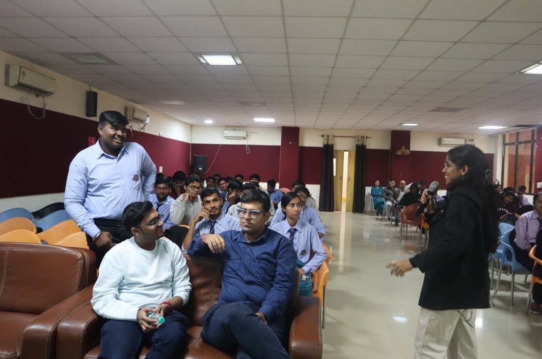
Stepped out of my comfort zone today. Spoke. Shared. Grew. Progress > Perfection. #machinelearningtutorial #SheBuilds #1sttalk

Priya and Arjun have been dating for 6 months. One day, Priya notices something suspicious – Arjun has started coming home late, hiding his phone, and smiling a lot at his screen. Priya’s friend whispers, “Girl, 90% chance he’s cheating!” 😱 Priya panics. She remembers that in their city, only 5% of boyfriends actually cheat (thankfully rare!). So if cheating is so rare, why is her friend so sure? This is exactly where Bayes’ Theorem comes to save the relationship (and your statistics exam). Let’s turn Priya into a detective using Bayes’ Theorem. Define the events: C → Arjun is cheating (bad news) ¬C → Arjun is NOT cheating (good news) S → Suspicious behaviour (late nights, hiding phone, secret smiles) We know from city gossip and surveys: P(C) = Probability a random boyfriend is cheating = 5% = 0.05 So P(¬C) = 1 – 0.05 = 0.95 P(S|C) = If he IS cheating, probability of suspicious behaviour = 90% = 0.90 (cheaters are usually bad at hiding it) P(S|¬C) = If he is NOT cheating, probability of suspicious behaviour anyway = 20% = 0.20 (maybe he’s planning a surprise birthday party, or just addicted to Candy Crush) Now Priya sees the suspicious behaviour (S happened). She wants to know: Given that he’s acting suspicious, what’s the actual probability he’s cheating? That is: P(C|S) = ? Bayes’ Theorem to the Rescue! The magic formula: P(C|S) = [P(S|C) × P(C)] / P(S) Where P(S) = total probability of seeing suspicious behaviour (whether cheating or not). P(S) = P(S|C)×P(C) P(S|¬C)×P(¬C) = (0.90 × 0.05) (0.20 × 0.95) = 0.045 0.190 = 0.235 (23.5%) Now plug into Bayes: P(C|S) = (0.90 × 0.05) / 0.235 = 0.045 / 0.235 ≈ 0.191 or 19.1% Even though the suspicious signs are strong (90% of cheaters show them), and even though Priya saw those signs… there’s only a ~19% chance Arjun is actually cheating! Priya takes a deep breath, confronts Arjun calmly…and finds out he was secretly learning guitar to serenade her on their 6-month anniversary. ❤️ #machinelearningtutorial

How did we go from if/else rules to neural networks? 1. Rule-based programming Great when the world is predictable. You cannot write a rule for every possibility. #machinelearningtutorial #NeuralNetworks #machinelearningforbeginners

France’s unemployment rate in Q3 2025 inched up to 7.7% from 7.6% in Q2 2025, with continuing rising unemployment for half year AJ Economy Trend - France Down due to continuous increase in unemployment for the past 6 months France’s unemployment rate in Q3 2025 inched up to 7.7% from 7.6% in Q2, the highest since Q3 2021 but still well below its 2015 peak. The number of unemployed rose by 44,000 to 2.4 million, leaving the rate 0.3 percentage points higher than a year earlier. By age, joblessness dropped for youth 15–24 (to 18.8%) but rose for 25–49 (7.1%) and 50 (5.1%). Male and female unemployment are now equal at 7.7%, after a 0.3-point rise for women. Despite the uptick, labor-market participation remains strong: the employment rate for ages 15–64 is 69.4%, near a record high, with full-time (57.6%) and part-time (11.8%) employment both stable. The activity rate is 75.2%, well above pre-pandemic levels, while long-term unemployment (1.8%) and underemployment (4.4%) were unchanged. #France #Europe #UnemploymentRate #Recession #AIBubble #AI #artificial_intelligence #machinelearningtutorial ajfinancialmarket.com

🚀 Browser Control With AI: Automate Anything in Minutes! If you’ve ever wished your browser could just do the work for you—open tabs, fill forms, click buttons, search, gather data—you’re going to love this. In my latest video, I show how to combine Google Gemini with the browser-use Python tool to automate Chrome using nothing but natural language. No complex scripts. No manual clicking. Just: “Open this page. Search for that. Extract this. Submit the form.” Watch here: youtu.be/z18qJyWAqh8?si=uTjp… #machinelearningprojects #machinelearningtutorial #machinelearningpython

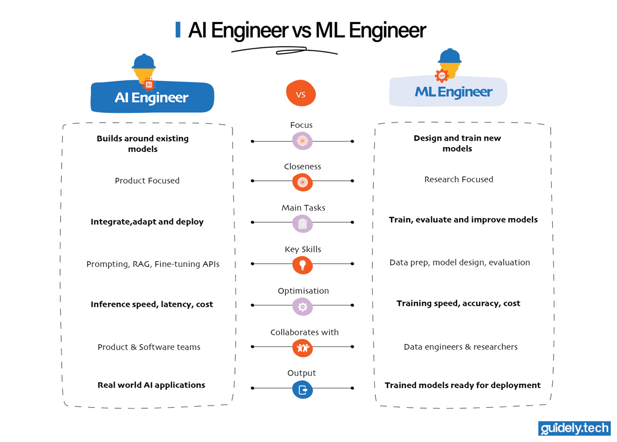
Two paths, same mission: build smarter systems. Which side do you find yourself leaning toward? #machinelearningtutorial #artificial_intelligence

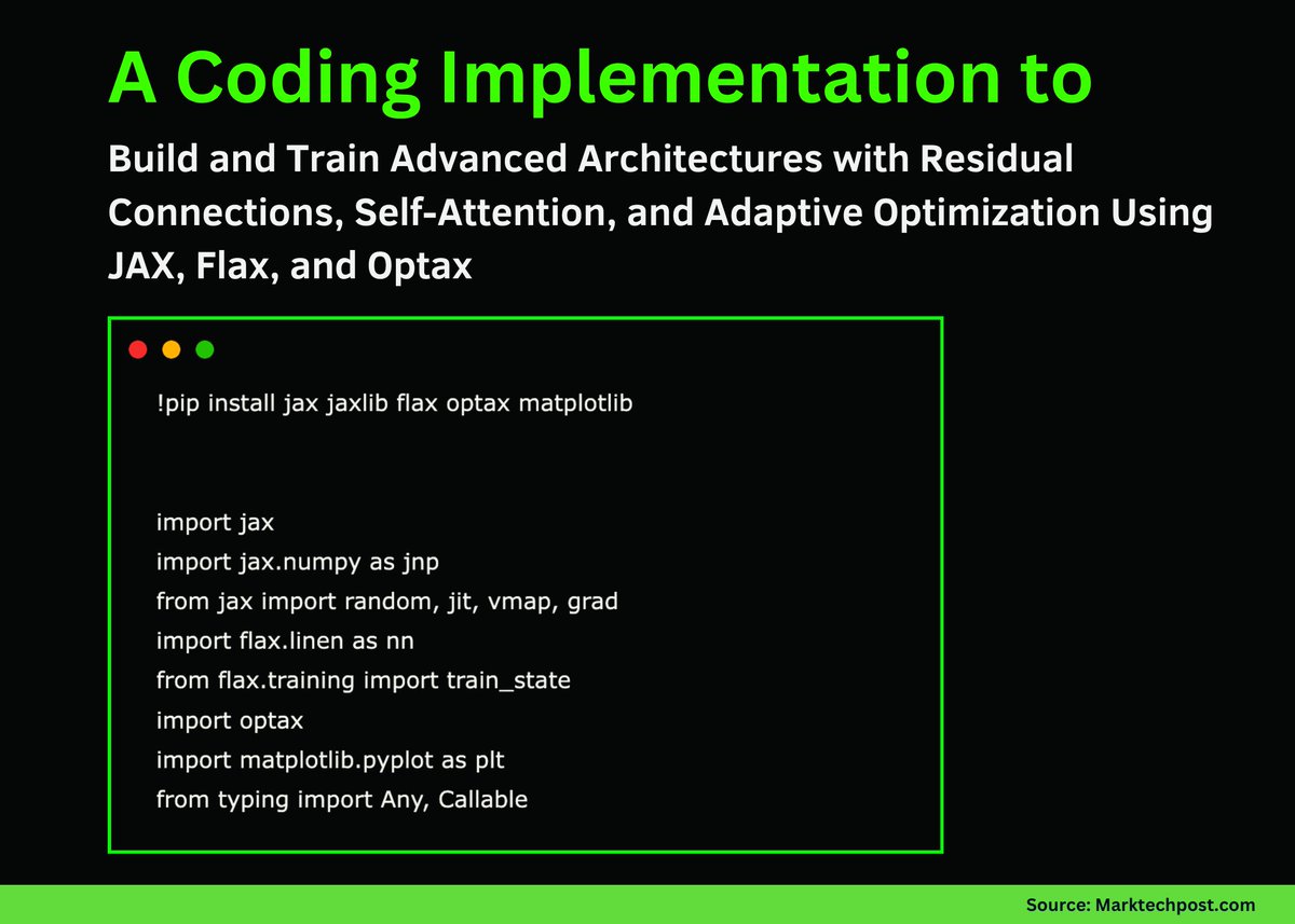
A Coding Implementation to Build and Train Advanced Architectures with Residual Connections, Self-Attention, and Adaptive Optimization Using JAX, Flax, and Optax In this tutorial, we explore how to build and train an advanced neural network using JAX, Flax, and Optax in an efficient and modular way. We begin by designing a deep architecture that integrates residual connections and self-attention mechanisms for expressive feature learning. As we progress, we implement sophisticated optimization strategies with learning rate scheduling, gradient clipping, and adaptive weight decay. Throughout the process, we leverage JAX transformations such as jit, grad, and vmap to accelerate computation and ensure smooth training performance across devices. Check out the FULL CODES here: github.com/Marktechpost/AI-T… Tutorial: marktechpost.com/2025/11/10/… #machinelearningprojects #machinelearningtutorial #machinelearningcode #machinelearningforbeginners #DataScientist #datasciencetutorials

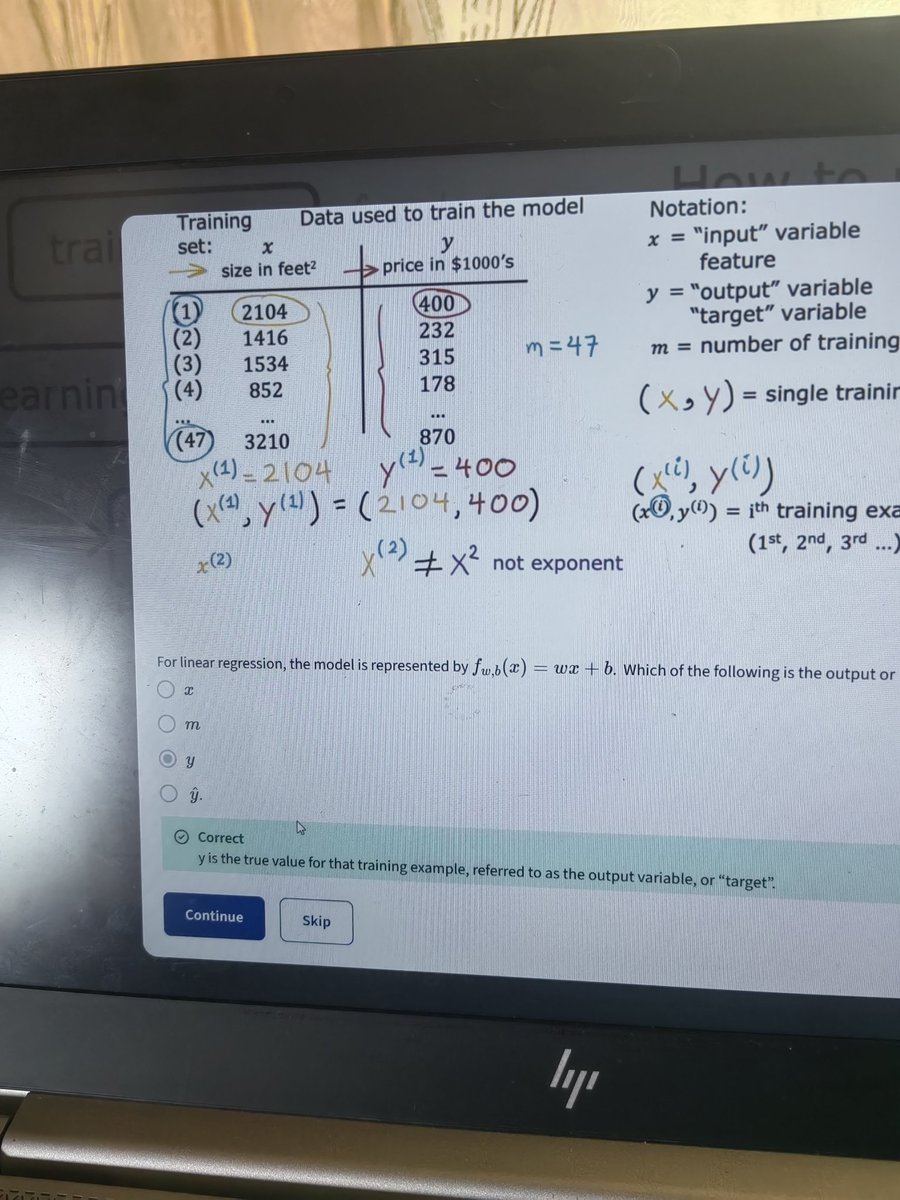
What did you learn today? 🤔 I studied on linear regression models, they are types of regression models that fits a straight line unto data. 📙 🖋️ I'm not done learning tho, my laptop is dead and I'm about to go play football. 😁💃 #machinelearningtutorial

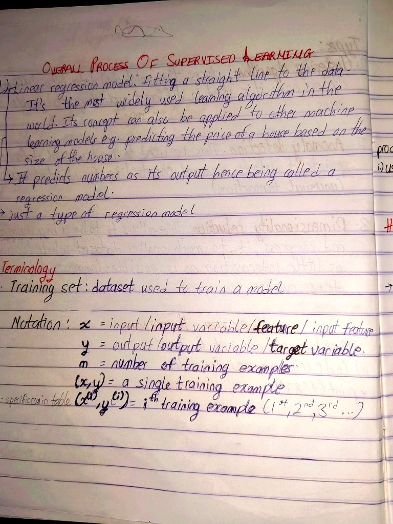
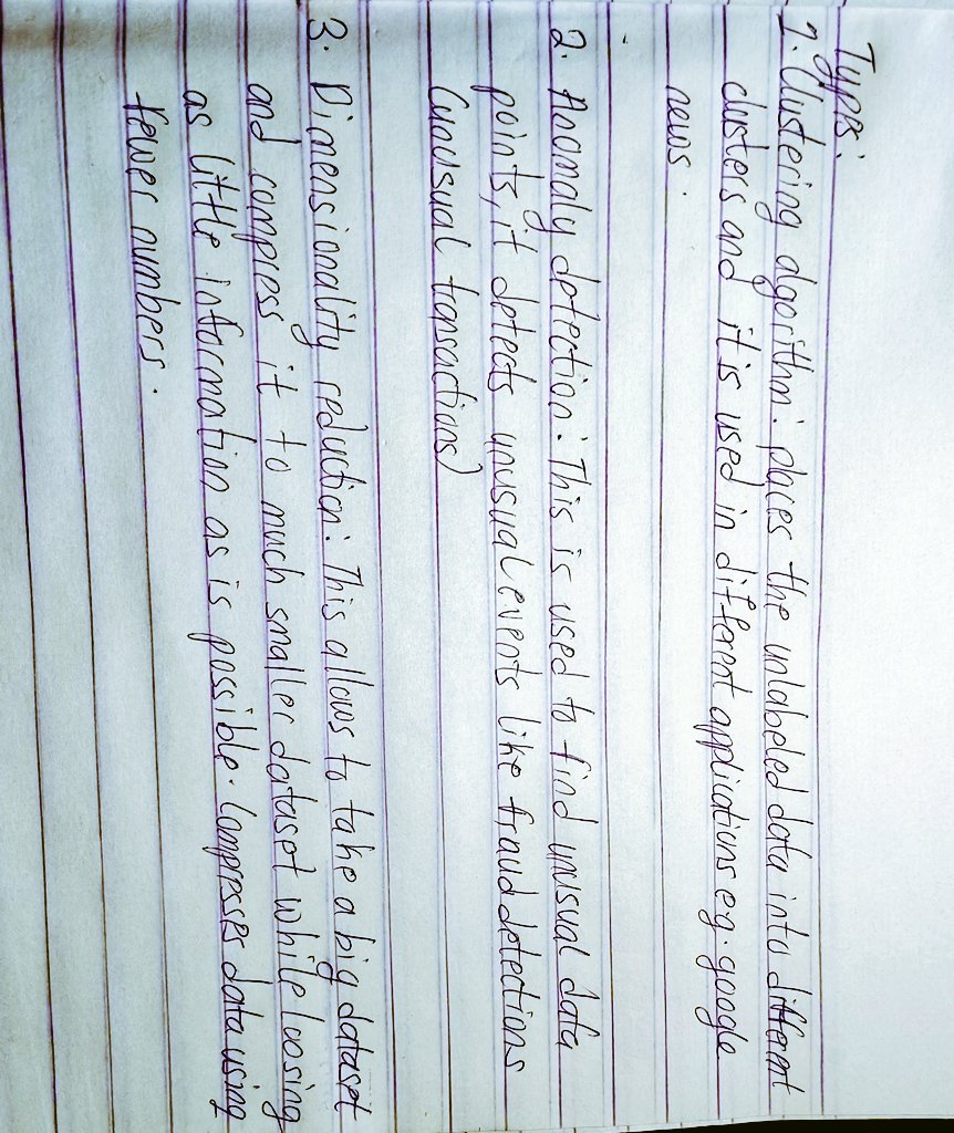
Learnt about the types of unsupervised learning today. 🤭 Am I the only one who struggles to post on Social media?🥲 I've detoxified so much that going from only WhatsApp to WhatsApp, X and LinkedIn feels overwhelming.😪 BTW, how's y'all academics going? #machinelearningtutorial

For the next 24 hours my course "Machine Learning Bootcamp for Complete Beginners" is 90% OFF regular price. Link: azamsharp.teachable.com/p/az… Coupon: 90OFF #machinelearningtutorial #machinelearning #ai

Hard work pays off as our latest review article summarizing the latest uses of #artificial_intelligence techniques in the field of #Endocrinology got published in #IndianJournalofEndocrinologyandMetabolism. Additionally, we have elucidated the various AI techniques for all readers. Congratulations to all my co-authors for their effort and special thumps up to #Minal and #Soubhik for their stupendous efforts. @j_metb @IndiaESI @AiimsKalyani #machinelearningtutorial #artificial_intelligence

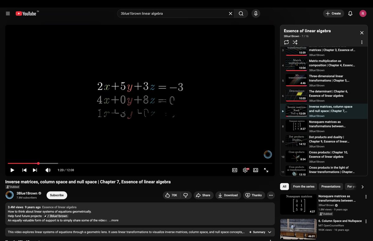
Alright floks completed this playlist. Next step is to complete Gilbert strang’s playlist.. And try to go with his book sbs. #machinelearningtutorial #LinearAlgebra #machinelearningforbeginners Thank you guys.. @herooffjustice @sayanreply

Gm Gm nerds.. Can I complete this??… #machinelearningtutorial #machinelearningforbeginners #LinearAlgebra

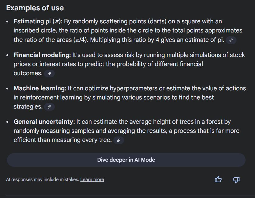
Learnt about the monte carlo method today.😌👍 Need to brush up my Statistics knowledge asap. #Python #machinelearningtutorial #11WeeksOfCode

DataHaven class day ten🎃 List of Content Model Evaluation & Metrics: Measuring AI Intelligence MLOps: From Model to Production Data Drift & Model Maintenance: Keeping Models Accurate #DataHaven #Crypto #machinelearningtutorial #artificial_intelligence

Give us 2 minutes and we will help you understand how a learning algorithm works! Learning algorithm ← (input X: cat image) → (output Ŷ: probability it’s a cat) Inside the learning algorithm, three parts work together: #machinelearningtutorial #artificial_intelligence