
Joined April 2016
- Tweets 4,455
- Following 3,444
- Followers 1,496
- Likes 11,726
215 Photos and videos


Pinned Tweet

First work-related trip (Paris) since covid started. Had one evening to walk around the beautiful latin quarter. Pantheon and crypt were spectacular.
13

Today, we share a breakthrough on the planar unit distance problem, a famous open question first posed by Paul Erdős in 1946.
For nearly 80 years, mathematicians believed the best possible solutions looked roughly like square grids.
An OpenAI model has now disproved that belief, discovering an entirely new family of constructions that performs better.
This marks the first time AI has autonomously solved a prominent open problem central to a field of mathematics.
1,200
3,917
26,778
13,580,493
Anastasia Brovkin | WearAMask | TA@NMA2020 retweeted

20 Dec 2025
Fascinating paper just published in Science.
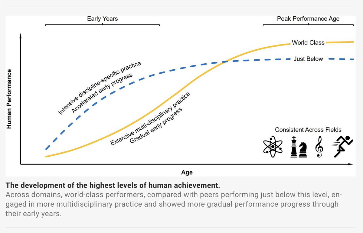
The authors analyze the career trajectories of top performers across multiple domains, including Nobel laureates, elite chess players, Olympic gold medalists, and more.
Their central finding challenges a common belief.
Intensive, single-discipline training at a young age does confer an early advantage, but this advantage fades over time.
By contrast, individuals exposed to multidisciplinary practice early in life tend to start more slowly. Yet, over the long run, they are more likely to reach world-class performance, eventually overtaking early specialists, who often plateau just below the very top.
An important reminder that breadth early on can be a powerful investment in long-term excellence.
Link to the paper in the first reply.
207
2,498
12,507
1,813,073
Anastasia Brovkin | WearAMask | TA@NMA2020 retweeted

28 Sep 2025
Individual researchers do not have attention mechanisms over the whole scientific literature. As a result, you get reinvention, even within the same subfield. It is exacerbated when the relevant was done much earlier. It is often exacerbated by the field not putting much emphasis on scholarship, and by conference reviewing, but it would happen anyway.
28 Sep 2025

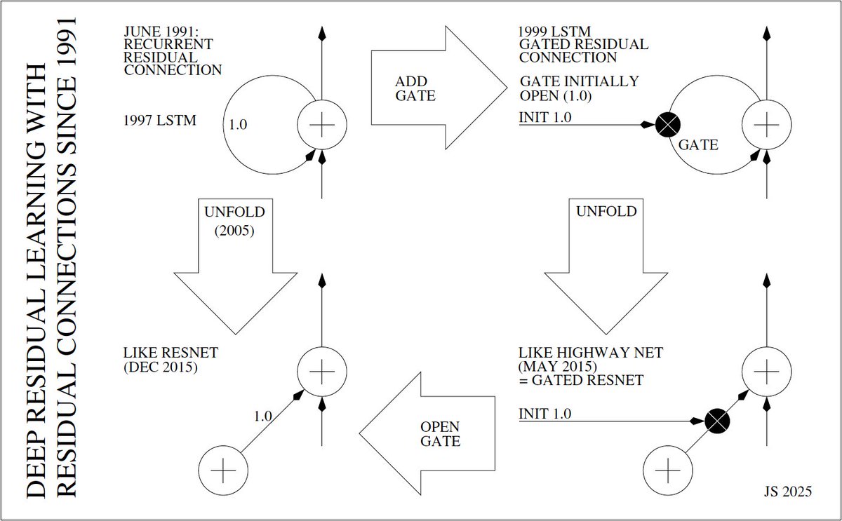
The most cited paper of the 21st century is on deep residual learning with residual connections. Who invented this? Timeline:
★ 1991: @HochreiterSepp solves vanishing gradient problem through recurrent residual connections (weight 1.0)
★ 1997 LSTM: plain recurrent residual connections (weight 1.0)
★ 1999 LSTM: gated recurrent residual connections (gates initially open: 1.0). With Felix Gers & Fred Cummins.
★ 2005: unfolding LSTM—from recurrent to feedforward residual NNs. With Alex Graves.
★ May 2015: very deep Highway Net—gated feedforward residual connections (initially 1.0). With @rupspace and Klaus Greff.
★ Dec 2015: ResNet—like an open-gated Highway Net (or an unfolded 1997 LSTM).
Details:
★ 1991: Sepp Hochreiter introduced residual connections for recurrent NNs (RNNs) in a diploma thesis (June 1991) [VAN1] supervised by Schmidhuber, at a time when compute was about 10 million times more expensive than today (2025). His recurrent residual connection was mathematically derived from first principles to overcome the fundamental deep learning problem of vanishing or exploding gradients, first identified and analyzed in the very same thesis [VAN1][DLP][DLH].
Like most good things, the recurrent residual connection is very simple: a neural unit with the identity activation function has a connection to itself, and the weight of this connection is 1.0.
That is, at every time step of information processing, this unit just adds its current input to its previous activation value. So it's just an incremental integrator. This simple setup ensures constant error flow in deep gradient-based RNNs: errors can be backpropagated [BP1-4][BPTT1-2] through such units for millions of steps without vanishing or exploding [VAN1], since according to the 1676 chain rule [LEI07-21b][L84] by Leibniz, the relevant multiplicative first derivatives (and their weights) are always 1.0.
Note that previous self-connections with real-valued weights other than 1.0 [MOZ] are not residual connections. Only 1.0 weights neutralize the vanishing/exploding gradient problem [VAN1]. However, almost residual connections with weights close to 1.0 are still acceptable in many applications. For example, a weight of 0.99 reduces an error signal backpropagated for 100 time steps (or virtual layers [BPTT1-2]) by an acceptable factor of 0.99100 ~ 37%. A weight of 0.9, however, yields only 0.9100 ~ 0.0027%.
Note that the additive weight changes of the earlier unnormalized linear Transformer (March 1991) [FWP0][ULTRA][FWP] represent a dual way of overcoming the vanishing gradient problem [FWP].
★ 1997 LSTM: plain recurrent residual connections (weight 1.0)
Recurrent residual connections (see above) are a defining feature of what was called Long Short-Term Memory (LSTM) in a 1995 tech report [LSTM0]. The subsequent LSTM journal paper (1997) [LSTM1] has become the most cited AI paper of the 20th century [MOST]. The LSTM core units with residual connections (weight 1.0) were called constant error carrousels (CECs) [LSTM1]. They are the very reason why LSTM can deal with very long time lags (hundreds or thousands of time steps) between inputs and target outputs. This became essential for processing speech and language [DL4][DLH].
★ 1999 LSTM: gated recurrent residual connections (gates initially open: 1.0)
Sometimes it is useful to let an NN modulate its residual connections through adaptive multiplicative gates, such that it can learn to reset itself. This was done in the 1999 LSTM variant [LSTM2,2a] that has become known as the vanilla LSTM. Its so-called forget gates were initialised by 1.0, such that they were open, to let the LSTM start out with plain residual connections (weight 1.0).
Over time, the 1999 LSTM could learn when to close those gates, thus temporarily shutting down the constant error flow, e.g., to focus on new tasks. This reintroduces the vanishing gradient problem [VAN1], but in a controlled way. This work was conducted by Schmidhuber's PhD student Felix Gers and his postdoc Fred Cummins.
★ 2005: unfolding LSTM - from recurrent to feedforward residual NNs
The backpropagation through time (BPTT) algorithm [BPTT1-2][BP1-4] unfolds the sequence-processing LSTM such that it becomes a deep feedforward NN (FNN) with a virtual layer for every time step of the observed input sequence. Until 2004, the gradients of LSTM's constant error carrousels (CECs) were often computed by a forward method called RTRL, instead of the more storage-consuming BPTT [BPTT2][RTRL24] (back then, computational hardware was 10,000 times more expensive and much more limited than today).
In 2005, however, Schmidhuber's PhD student Alex Graves started focusing on BPTT [LSTM3]. Here the recurrent residual connections in the CECs become feedforward residual connections (weight 1.0) in a deep residual FNN, typically many times deeper than the unfolded FNNs of previous gradient-based RNNs, thus making LSTM many times deeper than previous RNNs. That's why LSTM can deal with much longer time lags (hundreds or thousands of time steps) between relevant observations [DL4].
In the unfolded RNN, the resulting FNN weights are shared across time, but this makes no difference whatsoever for the residual connections: the weights of all residual connections in all RNNs and FNNs are tied to 1.0 anyway. Otherwise they wouldn't be residual connections. Whether or not the weights are shared between layers, gradients must still be propagated through many layers; hence the core role of residual connections is identical in both unfolded residual RNNs and residual FNNs (see below).
In RNNs, each time step/virtual layer allows for a new input and a new error signal/loss, unlike in standard FNNs. This is not an issue here. For example, in some of the original experiments designed to show LSTM’s superiority (1995-1997) [LSTM0-1], there is a sequence classification loss only at the very end of each input sequence, and the error really has to travel all the way back to the first input, which is the one that makes all the difference. Again, the residual parts of the unfolded residual RNN and residual FNNs (see below) are essentially the same.
★ May 2015: deep Highway Net - gated feedforward residual connections
While supervised LSTM RNNs had become very deep in the 1990s through residual connections, backpropagation-based FNNs had remained rather shallow until 2014: they had at most 20-30 layers or so, despite massive help through fast GPU-based hardware [MLP1-3][DAN,DAN1][GPUCNN1-9].
Since depth is essential for deep learning, the principles of deep LSTM RNNs were transferred to deep FNNs. In May 2015, the resulting Highway Networks [HW1][HW1a] (later called "gated ResNets") were the first working really deep gradient-based FNNs with hundreds of layers, over ten times deeper than previous FNNs. They worked because they adapted the 1999 LSTM principle of gated residual connections [LSTM2] from RNNs to FNNs. This work was conducted by Schmidhuber's PhD students Rupesh Kumar Srivastava and Klaus Greff.
Let g, t, h, denote non-linear differentiable functions of real values. Each non-input layer of a Highway NN computes g(x)x t(x)h(x), where x is the data from the previous layer.
The crucial residual part is the g(x)x part: the gates g(x) are typically initialised to 1.0 (like the forget gates of the 1999 LSTM above), to obtain plain residual connections (weight 1.0) which allow for very deep error propagation like in LSTM's unfolded CECs - this is what makes Highway NNs so deep.
So the initialised Highway NN starts out with very deep error propagation paths like the later ResNet (see below). However, depending on the application, it can learn to temporarily remove the residual property of some of its residual connections in a context-dependent way, provided this improves performance. (To reduce the number of learnable parameters, the oldest Highway Net paper [HW1] actually focused on the special case g(x) = 1 - t(x) where t(x) was initialized close to 0 such that during the forward pass each layer essentially just copied its input, resulting in backpropagated error derivatives very close to 1.0 - a common practice in today's deep NNs.)
★ Dec 2015: ResNet - like open-gated Highway Net (or unfolded 1997 LSTM)
Setting the Highway NN gates of May 2015 [HW1][HW1a] to 1.0 at all times (not just in the initial phase of training) effectively gives us the plain Residual Net or ResNet published 7 months later [HW2]. This open-gated variant of the Highway Net [HW1] is essentially a feedforward variant of the 1997 LSTM [VAN1][LSTM1], while the earlier Highway Net is essentially a gated ResNet and a feedforward variant of the 1999 LSTM [LSTM2]. (The term "residual" was apparently adopted from signal processing and control theory.)
Recall that the gates of the residual connections in Highway Nets are typically initialised to be open anyway, like in the 1999 LSTM. The network's training process can then decide to keep the gates open, or selectively close them if this improves performance. That is, the residual part of the Highway Net is initialized to be like the residual part of the later ResNet. That's what makes it so deep.
ResNets made a splash when they won the ImageNet 2015 competition [IM15]. Highway Nets perform roughly as well as ResNets on ImageNet [HW3].
The residual parts of a ResNet look essentially like those of an unfolded 1997 LSTM (or of an initialised, open-gated 1999 LSTM).
The ResNet paper [HW2] calls the Highway Net [HW1] "concurrent," but it wasn't: the ResNet was published 7 months later. The ResNet paper mentions the problem of vanishing/exploding gradients, but fails to mention that Sepp Hochreiter first identified it in 1991 and derived the solution: residual connections [VAN1]. The ResNet paper cites the earlier Highway Net in a way that does not make clear that ResNets are essentially open-gated Highway Nets, and that the gates of residual connections in Highway Nets are initially open anyway, such that Highway Nets start out with standard residual connections like ResNets. A follow-up paper by the ResNet authors suffered from design flaws leading to incorrect conclusions about gated residual connections [HW25b].
Note again that a residual connection is not just an arbitrary shortcut connection or skip connection (e.g., 1988) [LA88][SEG1-3] from one layer to another! No, its weight must be 1.0, like in the 1997 LSTM, or in the 1999 initialized LSTM, or the initialized Highway Net, or the ResNet. If the weight had some other arbitrary real value far from 1.0, then the vanishing/exploding gradient problem [VAN1] would raise its ugly head, unless it was under control by an initially open gate that learns when to keep or temporarily remove the connection's residual property, like in the 1999 initialized LSTM, or the initialized Highway Net.
Highway NNs showed how very deep FNNs can be trained by gradient descent. This is now also relevant for Transformers [ULTRA][TR1] and other NNs. In 2021, the US Patent Office granted a patent for Highway Nets (= gated ResNets) to our AI company NNAISENSE.
As I have often pointed out: deep learning is all about NN depth [DL1][DLH][MIR]. LSTMs brought essentially unlimited depth to supervised RNNs; Highway NNs brought it to FNNs. Remarkably, LSTM has become the most cited NN of the 20th century; the open-gated Highway Net variant called ResNet the most cited NN of the 21st [MOST]. The basic LSTM principle of constant error flow through residual connections is central not only to deep RNNs but also to deep FNNs. And it all dates back to 1991 [MIR].
REFERENCES
All references in: J. Schmidhuber. Who invented deep residual learning? Technical Report IDSIA-09-25, IDSIA, September 2025.
people.idsia.ch/~juergen/who…
9
11
253
62,409
Anastasia Brovkin | WearAMask | TA@NMA2020 retweeted

3 Feb 2025
Really excited to share our new preprint "Geometric influences on the regional organization of the mammalian brain" with @AFornito and a superstar 17-person team! (1/n)
biorxiv.org/content/10.1101/…
1
36
91
13,068
Anastasia Brovkin | WearAMask | TA@NMA2020 retweeted

14 Jan 2025
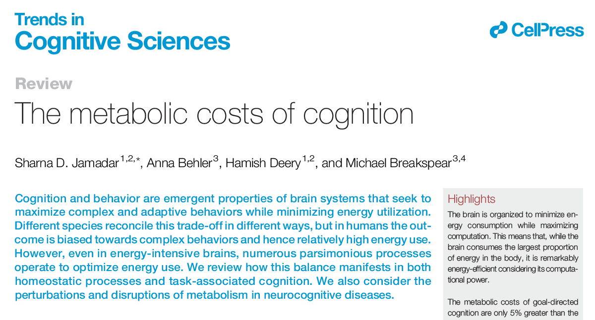
The metabolic costs of cognition
Review by Sharna D. Jamadar (@SharnaJamadar), Anna Behler (@Anna_NeuroSci), Hamish Deery (@DeeryHamish), & Michael Breakspear (@DrBreaky)
Free access before March 4: tinyurl.com/47c9n65w
3
113
393
89,285
Anastasia Brovkin | WearAMask | TA@NMA2020 retweeted

26 Nov 2024
Everyone using RNNs to model the brain has their favorite activation function: sigmoid, tanh, ReLU. But does it matter which one you choose? Turns out it does! Activation functions affect representations, dynamics, and circuit solutions. biorxiv.org/content/10.1101/…
@TolmachevPavel2
26 Nov 2024

RNNs are often used as a model for exploring how the brain may solve specific tasks. In a new preprint, we show that, depending on the architecture, RNNs find different circuit solutions, behaving differently when exposed to novel stimuli.
biorxiv.org/content/10.1101/…
@EngelTatiana
1
22
131
14,562
Anastasia Brovkin | WearAMask | TA@NMA2020 retweeted

2 Oct 2024
Big news! The fly connectome is featured on the cover of a special edition of Nature.
This is all possible thanks to the collaboration of 292 members of The FlyWire Consortium!
nature.com/immersive/d42859-…
Check out the thread for an overview of the 9 #flywire papers published today

9
236
530
190,195
Anastasia Brovkin | WearAMask | TA@NMA2020 retweeted

2 Oct 2024
A simple statistical model capturing only pairwise interactions between brain regions is sufficient to reproduce key features of whole-brain dynamics.
Read go.aps.org/3ZPLJM4
#Complexsystems #Neuroscience
5
105
442
23,422
Anastasia Brovkin | WearAMask | TA@NMA2020 retweeted
9 Aug 2024
A new method of detecting criticality from time-series data outperforms conventional metrics in the presence of variable noise levels for both simulated systems and real neural recordings.
Read go.aps.org/3WBjcXf
#PRXjustpublished #PRXopenaccess #PRXComplexSystems

24
126
18,615
Anastasia Brovkin | WearAMask | TA@NMA2020 retweeted

22 Jul 2024
The brain is metabolically hungry but most accounts of cognition do not consider the energy cost of neural activity
Here we review the metabolic budget of neural homeostasis cognition; associated evolutionary constraints; plus disturbances in disease
osf.io/preprints/osf/m5jze
11
124
417
30,479
Anastasia Brovkin | WearAMask | TA@NMA2020 retweeted

24 Jun 2024
Our book on diffusion MRI tractography is now out: shop.elsevier.com/books/hand…
Enjoy!

40
135
8,405
Anastasia Brovkin | WearAMask | TA@NMA2020 retweeted

22 Jun 2024
At #OHBM2024 I'll be presenting my work where I used generative network models to explore the constraints on connectome formation. Come see my poster (#1530, Wednesday/Thursday) to learn what I wish I had known 4 years ago when doing my PhD :)

1
18
94
8,835
Anastasia Brovkin | WearAMask | TA@NMA2020 retweeted

20 Jun 2024
🇬🇧 Vote on #ChatControl postponed – a triumph in our fight to defend the digital privacy of correspondence and secure encryption. 💪 Thank you!
But the next attempt will come. The critical governments need to get their act together now:
patrick-breyer.de/en/chat-co…

ALT Celebrating emoji. Text: "Vote cancelled Chat Control averted! (for now) Your resistance was successful. Thank you! Celebrate, connect, prepare for the next attack! #ChatControl patrick-breyer.de/en" Logo of the European Pirates
26
237
717
76,624
Anastasia Brovkin | WearAMask | TA@NMA2020 retweeted

18 Jun 2024
Nach dem Messenger Signal hat sich auch Threema deutlich gegen die #Chatkontrolle ausgesprochen. Kommt die Verordnung so, könnte er Europa verlassen netzpolitik.org/2024/chatkon…
9
318
658
28,062
Anastasia Brovkin | WearAMask | TA@NMA2020 retweeted

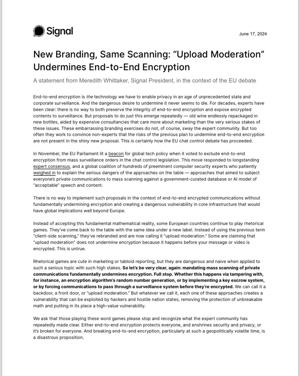
17 Jun 2024
📣Official statement: the new EU chat controls proposal for mass scanning is the same old surveillance with new branding.
Whether you call it a backdoor, a front door, or “upload moderation” it undermines encryption & creates significant vulnerabilities
signal.org/blog/pdfs/upload-…
200
3,720
7,858
2,030,176
Anastasia Brovkin | WearAMask | TA@NMA2020 retweeted

23 May 2024
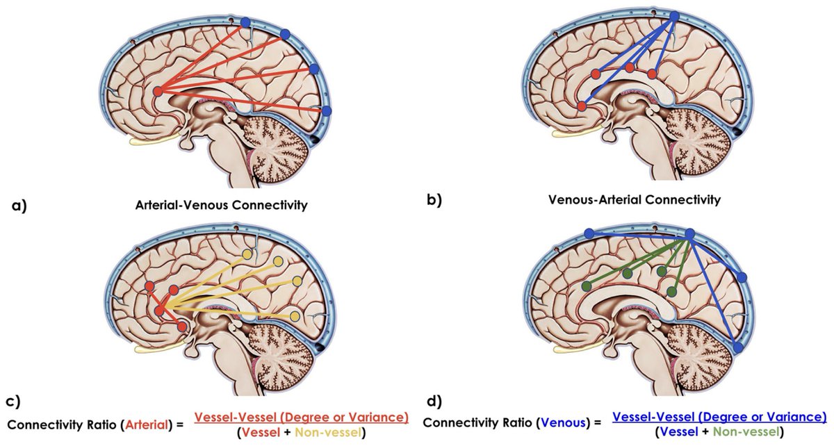
New paper in Imaging Neuroscience by Xiaole Z. Zhong, Yunjie Tong, and J. Jean Chen:
Assessment of the macrovascular contribution to resting-state fMRI functional connectivity at 3 Tesla
doi.org/10.1162/imag_a_00174
201
16
84
19,199
Anastasia Brovkin | WearAMask | TA@NMA2020 retweeted

15 Apr 2024
By insisting that every brain-behavior association study include hundreds or even thousands of participants, we risk stifling innovation. Smaller studies are essential to test new scanning paradigms.
By Emily S. Finn
thetransmitter.org/future-of…
2
50
126
59,627
Anastasia Brovkin | WearAMask | TA@NMA2020 retweeted

27 Mar 2024
Whole, healthy human brain data is now on the ABC Atlas!
Dataset incl. 3 million cells sampled from dissections from adult donors. Samples underwent snRNA sequencing and were clustered and categorized by neurotransmitter, region, and more.
ABC Atlas: portal.brain-map.org/atlases…
4
55
190
20,622
Anastasia Brovkin | WearAMask | TA@NMA2020 retweeted
9 Feb 2024
Undertaking inference on spatial brain maps?
Correspondence between maps?
Textures and other nuggets of gold buried within maps?
Spatiotemporal processes in dynamic maps (e.g. fMRI)?
Here is your method for non-parametric inference :-)
biorxiv.org/content/10.1101/…
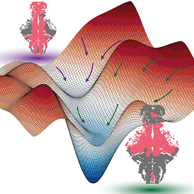
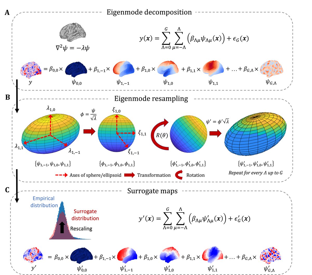
9 Feb 2024

Thrilled to present our preprint for a new brain null method (doi.org/10.1101/2024.02.07.5…) 🧠
Here we present "eigenstrapping", which exploits the intrinsic geometric constraints of the brain to generate surrogate brain maps with closely matched spatial autocorrelation.
More below 👇
2
19
92
9,971
Anastasia Brovkin | WearAMask | TA@NMA2020 retweeted

29 Jan 2024
We're hiring! New post-doc role at @Sydney_Uni with @jlizier and @bendfulcher focussed on whole-brain neuroimaging and some cool computational methods. Full app details here: usyd.wd3.myworkdayjobs.com/U…. To start in July 24. Feel free to reach out if you have Qs. Oh, and please RT!
2
77
96
24,060