

Jun 12
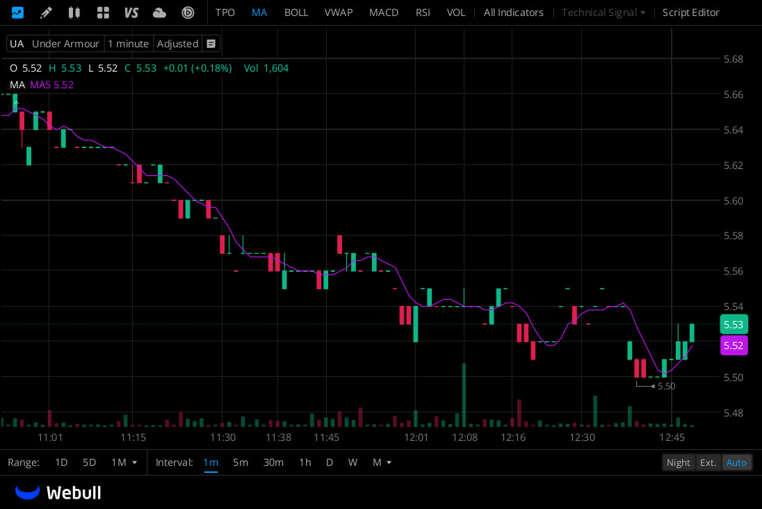
If you’re glued to the market all day but still can’t lock down solid trading opportunities,
consider following 👉@thomasHa80.
He’s dropped some really sharp market takes lately, including:
✅ $FNLC
✅ $CLLS
✅ $FNWD. His content’s definitely worth adding to your follow list.
58


Jun 8
Grand Chief Stewart Philip was paid approximately $930,000 tax free in the last year for which records are public. His organisation, the FNLC, says it’s co-governing BC.
He’s not an elite?
8
20
113
1,065

May 19
l’infériorité numérique initiale (environ 400 Français face à ~1 000 rebelles bien armés dans la ville).25
20 mai à l’aube : La deuxième vague (~233-250 parachutistes, dont la 4e compagnie, mortiers, reconnaissance) saute en renfort. Dans la journée, les parachutistes belges (opération Red Bean / Dragon Vert) atterrissent sur l’aéroport (déjà partiellement sécurisé par des paras zaïrois) et participent à la sécurisation et à l’évacuation. Kolwezi est globalement sous contrôle en fin de journée. Les combats et ratissages se poursuivent plusieurs jours.32
Bilan humain et militaire
•Côté français (2e REP) : 5 tués (les cinq légionnaires mentionnés précédemment) et une vingtaine de blessés. Quelques disparus ou tués à la mission militaire française.
•Côté rebelles (FNLC) : 250 à 400 tués, ~160 capturés. Nombreuses armes saisies (mortiers, mitrailleuses, roquettes, etc.).
•Civils : Plus de 100-170 Européens et plusieurs centaines d’Africains tués (avant et pendant l’opération). Plus de 2 000 à 2 800 Européens et des milliers d’Africains évacués et sauvés.16
L’opération s’achève officiellement vers le 22-23 mai, avec des opérations de sécurisation jusqu’à mi-juin.
Conséquences et héritage
L’opération Bonite est un succès militaire et humanitaire remarquable : un saut aéroporté audacieux à plus de 6 000 km de la France, avec effet de surprise décisif, malgré des conditions risquées (basse altitude, feu ennemi, fatigue des troupes). Elle reste une référence dans l’histoire des opérations aéroportées modernes et renforce la réputation du 2e REP.
Politiquement, elle sauve le régime de Mobutu à court terme et marque une intervention occidentale dans le contexte de la Guerre froide en Afrique (contre l’influence cubaine et soviétique via l’Angola). Elle est parfois critiquée pour son aspect néocolonial, mais elle est surtout saluée pour avoir évité un massacre plus large.
Les cinq légionnaires tombés sont honorés chaque année par la Légion. Leur devise « More Majorum » (« À la manière de nos anciens ») incarne parfaitement leur engagement.
Cette bataille reste l’une des pages les plus glorieuses et tragiques de l’histoire récente de la Légion étrangère.💚❤️🫡


1
3
10
395
May 19
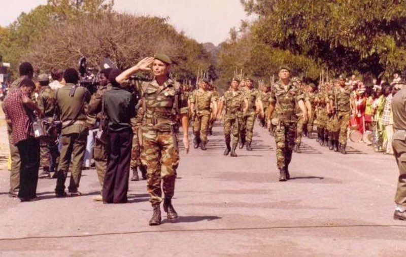
🪖🇫🇷la bataille de #Kolwezi (opération #Bonite / opération #Léopard),
mai 1978
Contexte géopolitique et historique
En #1978, le Zaïre (aujourd’hui République démocratique du Congo) est dirigé par le maréchal Mobutu Sese Seko, allié de l’Occident dans le contexte de la Guerre froide. La province du Shaba (ex-Katanga), riche en cuivre, cobalt, uranium et autres minerais, est vitale pour l’économie zaïroise et les intérêts occidentaux (notamment belges et français via l’entreprise Gécamines).
Les rebelles katangais du FNLC (Front national de libération du Congo, aussi appelés « Tigres katangais » ou Gendarmes katangais) sont d’anciens sécessionnistes des années 1960. Ils se sont réfugiés en Angola, où ils sont entraînés par les Cubains et armés par le bloc soviétique. Leur objectif : déstabiliser Mobutu et prendre le contrôle des richesses minières. C’est la deuxième guerre du Shaba (Shaba II).7
L’invasion et les massacres (13-18 mai 1978)
Le 13 mai 1978, environ 3 000 à 4 000 rebelles du FNLC envahissent Kolwezi, ville minière importante. Les forces armées zaïroises (FAZ) s’effondrent rapidement, souvent en fuyant ou en pillant elles-mêmes.
Les rebelles prennent le contrôle de la ville. Ils pillent, violent et massacrent. Des centaines de civils africains et plus d’une centaine d’Européens (principalement des techniciens belges et français) sont tués dans les jours suivants. Les estimations varient : entre 120 et 170 Européens et plus de 700 Africains massacrés au total pendant l’occupation. Des milliers d’autres civils se cachent dans les maisons, caves, greniers ou toits. Des scènes horribles sont rapportées : exécutions sommaires, mutilations, viols.15
Environ 2 000 à 2 800 Européens (et des milliers d’Africains) sont pris en otages ou bloqués. La situation devient une urgence humanitaire internationale.
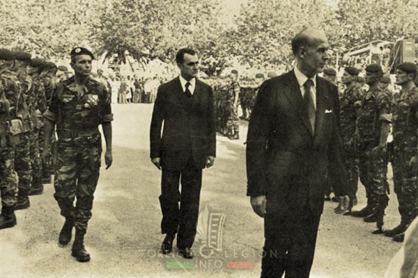
La décision française et la préparation
Alerté par les massacres et à la demande pressante de Mobutu, le président Valéry Giscard d’Estaing décide d’intervenir militairement pour sauver les otages. L’opération reçoit le nom de code Bonite (Léopard côté zaïrois). La mission est confiée au 2e Régiment étranger de parachutistes (2e REP), basé à Calvi (Corse), commandé par le colonel Philippe Erulin. C’est une unité d’élite, hautement entraînée pour les opérations aéroportées.3
Le régiment est mis en alerte le 17 mai. Dans la nuit du 17 au 18 mai, les légionnaires sont acheminés par avion (DC-8 français et C-130 américains) vers Kinshasa. Les colonels Yves Gras (mission militaire française) et Philippe Erulin préparent l’opération dans l’urgence.
Le saut et les combats (19-20 mai)
19 mai 1978, vers 15h30-15h40 (heure locale) : La première vague (environ 381 à 405 parachutistes des 1re, 2e et 3e compagnies éléments d’état-major) saute à basse altitude (environ 250 mètres) sur une zone de largage près de l’ancien aérodrome / hippodrome au nord de la vieille ville. Le saut se fait sous le feu ennemi. Six hommes sont blessés dès l’atterrissage. Un légionnaire isolé est tué et mutilé avant même de se libérer de son parachute.28
Dès leur arrivée au sol, les combats de rue sont violents et intenses. Les légionnaires progressent par petits groupes, neutralisent les positions rebelles (hôtel Impala, poste, hôpital, etc.), libèrent les otages cachés et stoppent des contre-attaques (notamment une colonne avec véhicules blindés à la gare). Des snipers français font des ravages. En quelques heures, les points stratégiques sont pris malgré👇🏻
1
4
16
727


Why is co-governance between BC and First Nations groups like @BCAFN, FNLC and @UBCIC an issue?
PLUS legal advisor, Geoff Moyse, KC, says in @WDiminishment it's about their inability to represent the public interest, and threats "indicating a willingness to engage in acts of civil disobedience."
withoutdiminishment.com/p/th… #bcpoli
2
3
7
451

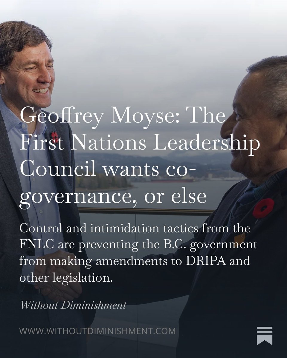
Geoffrey Moyse: The First Nations Leadership Council wants co-governance, or else
"A careful reading of UNDRIP leads to the inevitable conclusion that it is a UN-created recipe for the co-governance of this province by the FNLC."
withoutdiminishment.com/p/th…

1
6
12
1,634

May 5
France: les rebelles indépendantistes du FNLC sont-ils des terroristes ? rfi.fr/fr/france/20230804-fr…
1
3
88

May 5
British Columbia’s government is surrendering democratic control to the First Nations Leadership Council over DRIPA and UNDRIP, writes Geoffrey Moyse.
The FNLC demands zero changes to the law and threatens legal action, political pressure, and direct action if Premier Eby proceeds without their consent.
Instead of acting, the NDP has paused reforms for six months of negotiations, despite the urgent legal risks exposed by the Gitxaala court ruling.
UNDRIP as positive law hands unelected leaders veto power over legislation affecting Indigenous rights, creating endless litigation, uncertainty, and co-governance. This clashes with parliamentary sovereignty and the Constitution.
British Columbians deserve better than rule by consent of 2 percent of the population.
The latest in @WDiminishment.
withoutdiminishment.com/publ…
12
18
1,600

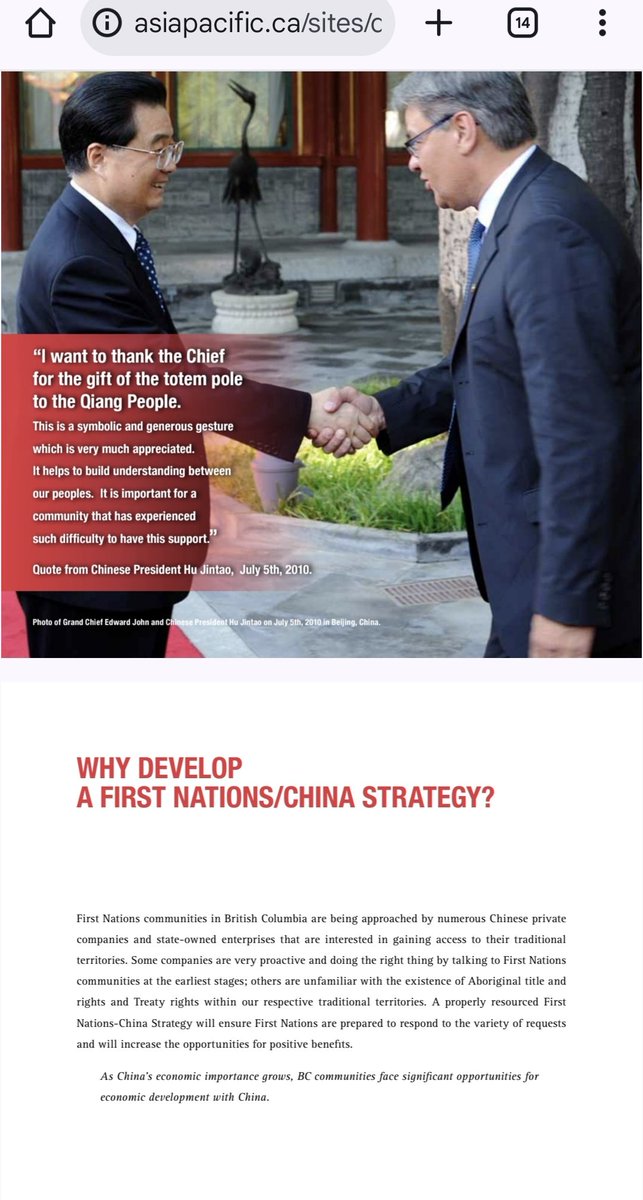
The First Nations Leadership Council FNLC - Energy and Mining Council The Union of BC Indian Chiefs, First Nations Summit and BC Assembly of First Nations has created sector specific councils working with China.


They just had a group of chiefs visit China. Should this not be a matter of national security? First Nations are literally planning a separation and allowing a foreign nation to step in.
They already have wealth sharing plans that do not include Canada. See the snapshots.


1
2
7
231

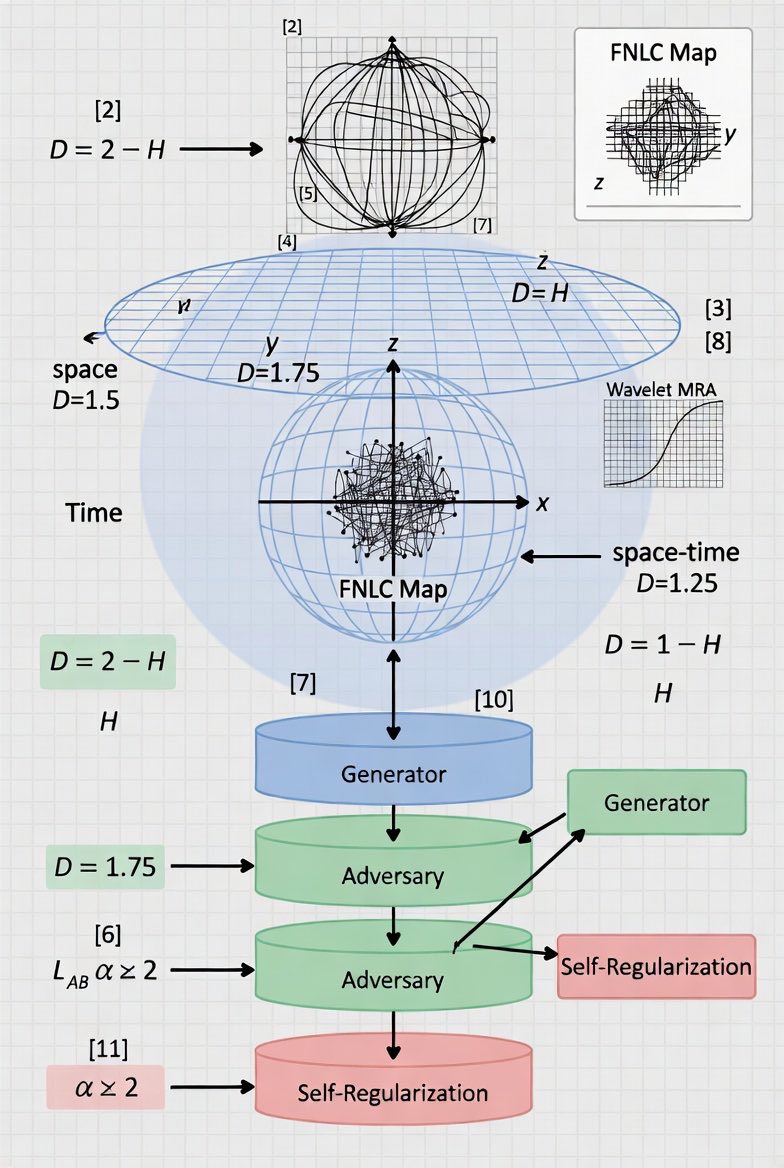
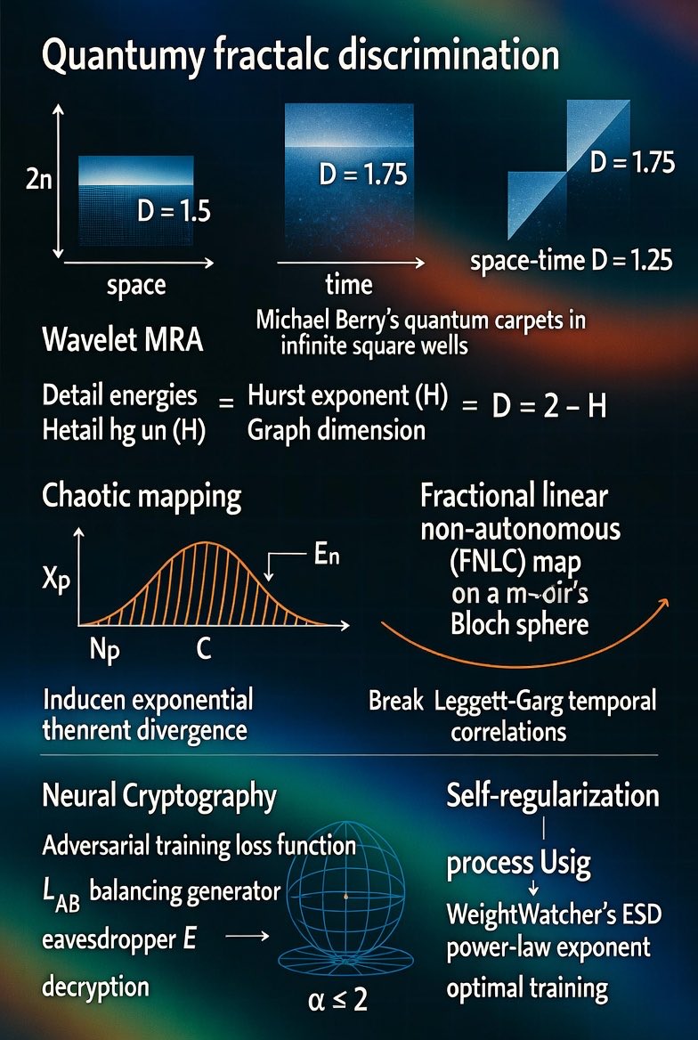
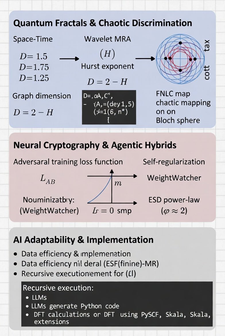
1. Quantum Fractals & Chaotic Discrimination
• Space-Time Dimensions: Uses Michael Berry's work on quantum carpets in infinite square wells, defining fractal dimensions for space (D=1.5), time (D=1.75), and space-time (D=1.25) [2].
• Wavelet MRA: Relates detail energies to the Hurst exponent (H) and graph dimension (D = 2 - H) [3, 4].
• Chaotic Mapping: Utilizes a fractional linear non-autonomous chaotic (FNLC) map on a Bloch sphere to induce exponential divergence and break Leggett-Garg temporal correlations [5, 6].
2. Neural Cryptography & Agentic Hybrids
• Adversarial Training: Uses a loss function (L_AB) that balances the generator's ability to create secure keys against an eavesdropper's (E) ability to decrypt them [7, 8].
• Self-Regularization: Uses WeightWatcher to monitor the Empirical Spectral Density (ESD) power-law exponent (α), where an ideal α ≈ 2 indicates optimal training without over- or under-fitting [9].
3. AI Adaptability & Implementation
• Data Efficiency: Prioritizes a small set of highly curated, high-fidelity workflows over massive synthetic datasets [10].
• Recursive Execution: LLMs generate Python code using PySCF and Skala extensions for Density Functional Theory (DFT) calculations, evaluating their own success and correcting errors dynamically [11].
To advance this discussion, do you want to deep-dive into the mathematics of the FNLC chaotic map, or would you prefer to explore how to physically implement the fidelity-aware scheduler in Python, JavaScript, and C ? In the context of the Parrish/Skala framework, "learning" does not refer to simple gradient descent on a dataset. Instead, it refers to hybrid adaptability: a combination of adversarial dynamics, spectral self-monitoring, and recursive agentic loops.
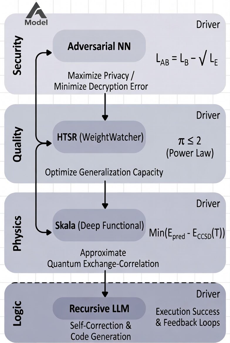
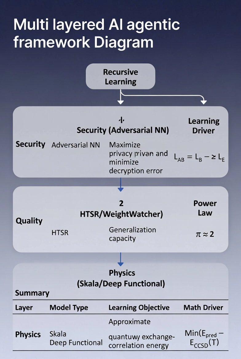
Below is an expansion on the three specific deep learning models and learning mechanisms outlined in this framework.
1. Adversarial Neural Cryptography (The "Competitive" Learner)
This model replaces standard encryption algorithms with neural networks (Alice, Bob, and Eve) that learn to encrypt and decrypt through adversarial competition.
• Architecture:
◦ Alice (A): Takes a plaintext P and key K, outputs ciphertext C.
◦ Bob (B): Takes C and K, tries to reconstruct P.
◦ Eve (E): Takes only C, tries to reconstruct P.
• The Learning Mechanism (Loss Functions): The system does not minimize a single static error. Instead, it optimizes a minimax game defined by the compound loss function L_AB.
◦ Bob’s Loss (L_B): Measures communication success (L1 distance between Bob's guess and real P). L_B = (1/N) Σ |P_i - B(C,K)_i|
◦ Eve’s Loss (L_E): Measures interception success. The adversarial component forces Alice to maximize this loss (making Eve fail). L_E = E[L1(P, E(C))]
◦ Total Adversarial Loss (L_AB): L_AB = L_B - λ L_E. Here, λ is a hyperparameter regulating the "privacy budget." If λ is too low, Alice ignores Eve; if too high, Alice creates encryption so chaotic even Bob cannot decrypt it. [1, 2]
2. Heavy-Tailed Self-Regularization (The "Diagnostic" Learner)
In this framework, agents use WeightWatcher to monitor how well they are learning without needing a test set. This is based on the Heavy-Tailed Self-Regularization (HTSR) theory, which treats neural network layers as statistical mechanical systems.
• The Model (ESD Power Law): Instead of looking at accuracy, the agent calculates the Empirical Spectral Density (ESD) of the layer weight matrices (eigenvalues λ of W^T W). ρ(λ) ~ λ^{-α}
• The Metric (α): The exponent α acts as a "thermometer" for the learning process:
◦ α > 6: Undertrained (Gaussian/Random matrix behavior).
◦ α ≈ 2: Optimal Learning. The model is at the "edge of chaos," balancing memorization (low rank) and generalization (heavy tails).
◦ α < 1.5: Over-correlated/Collapse.

6
3
127
Quantum Fractals & Chaotic Discrimination (Adaptability in Dynamics)
Infinite square-well carpets: space fractal dimension (D_space = 3/2), time (D_time = 7/4), space-time (D_space-time = 5/4) (Berry). Wavelet MRA: detail energies (E_j ∼ 2^{-jα}), Hurst (H = -α), graph dimension
[D = 2 - H.]
Chaos-mediated discrimination (FNLC map on Bloch sphere):
[f(z) = (2sz 1)/(2z s), s = i]
(yields exponential divergence; Leggett-Garg correlation (r_XY → 0) after waiting time τ(δ)).
Neural Cryptography & Agentic Hybrids (Direct AI/LLM Tie-In)
Adversarial training losses:
[L_B = 1/N Σ |P_i - B(C,K)_i|, L_E = E[L1(P, E(C))], L_AB = L_B - λ L_E.]
SETOL/HTSR monitors ESD power-law (ρ(λ) ∼ λ^{-α}) (ideal α ≈ 2); probit uncertainty (P(y=1|x) = Φ(x^T β)). Recursive LLMs enable executable code generation for state inspection/transforms.
Programming AI Adaptability for Agents and LLMs
Parrish’s threads advocate hybrid, data-efficient programming for adaptability—echoing Skala’s two-stage training and Agency Efficiency Principle (quality workflows > raw scale). Agents/LLMs become “adaptable” via recursive/self-referential loops, tool-use (TPTU-style), fidelity-aware scheduling, and quantum-classical orchestration. Best practices: curate ~78 high-quality full-workflow examples (beats 10k synthetics); monitor via WeightWatcher for self-regularization; integrate quantum simulators (PySCF Skala) for chemistry agents.
Practical Implementation Sketch (Python/PyTorch Skala/PySCF Extensions)
# Hybrid Agentic LLM Skala-DFT for Scientific Adaptability
import torch
from pyscf import gto, scf
from skala.pyscf import SkalaKS
import weightwatcher as ww
# 1. Recursive LLM Agent (adaptability via code-gen self-correction)
class RecursiveAgent:
def __init__(self, llm):
self.llm = llm
self.history = []
def plan_and_execute(self, task, quantum_mol=None):
code_prompt = f"Generate PySCF Skala code for {task} with error correction."
plan = self.llm.generate(code_prompt)
try:
exec(plan)
mol = gto.M(atom=quantum_mol, basis="def2-tzvp")
ks = SkalaKS(mol, xc="skala-1.1")
e = ks.kernel()
self.history.append(e)
except Exception as err:
correction = self.adapt_via_weightwatcher(plan)
return self.plan_and_execute(task, quantum_mol)
return e
def adapt_via_weightwatcher(self, model_code):
watcher = ww.WeightWatcher(model=eval(model_code))
df = watcher.analyze(detX=True)
if df['alpha'].mean() < 1.8:
return "adjusted plan with α→2 regularization"
return model_code
# 2. QHPC Orchestration
# Fidelity-aware scheduler pseudocode:
# score = fidelity * (1 - latency_µs/4) * parallelism_factor
Adaptability Best Practices (Parrish-Style)
• Data Efficiency: 78 curated workflows > 10k samples.
• Monitoring: WeightWatcher probit heads for uncertainty; enforce ERG (det X ≈ 0).
• Hybrid Scaling: Embed Skala DFT calls in LLM agents for real-time molecular QM (reaction energies at hybrid accuracy, O(N) cost).
• Error Mitigation: Chaotic amplification Leggett-Garg witnesses; photonic cooling Lindbladian for hardware-in-loop agents.
• Extensions: Fork Skala GitHub GPU4PySCF; add recursive loops for long-horizon agentic behavior.
This framework—drawn directly from @kparrish51’s threads—makes AI agents/LLMs systematically improvable for quantum chemistry, materials discovery, and beyond. Parrish’s X threads serve as living, equation-rich reviews.

1
6
5
140

【🕵️インサイダー買い🇺🇸小型株🐤】
直近1週間分
$AXR AMREP
4月29日 主要株主が約13.9万ドル買い
5月1日 主要株主が約8.4万ドル買い
$AUID authID
4月29日 取締役2名が買い
約3.8万ドルと約15.1万ドル
$CBK Commercial Bancgroup
4月30日 EVPが約9.6万ドル買い
$CSTM Constellium
5月1日 取締役が約4.1万ドル買い
$EQBK Equity Bancshares
4月29日 取締役が約9.2万ドル買い
$FNLC First Bancorp
4月30日 取締役が約4.3万ドル買い


Low IQ investors still believe in randomness and the stock market alone, but the reality is that insider trading always wins.
8
428
Page 2 of 3
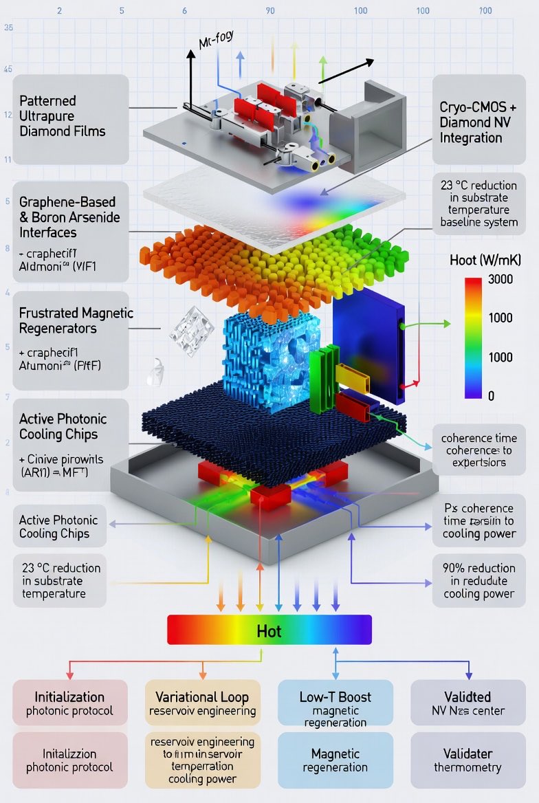
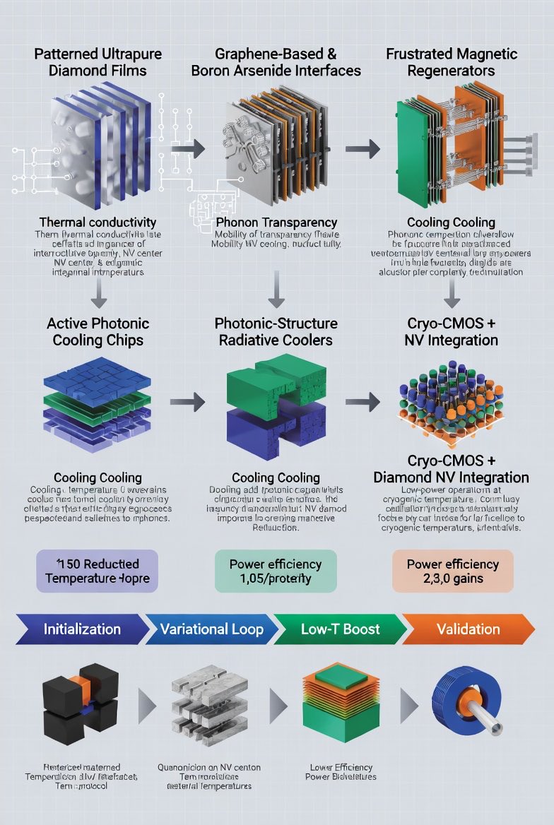
3. Best Materials for Optimized Cooling & Energy Efficiency (2026 State-of-the-Art): These materials are monolithically integrated into the BEOL photonic stack and replace theoretical placeholders with verified 2026 breakthroughs:
• Patterned Ultrapure Diamond Films (Rice University, 2026): Bottom-up overgrowth converts damaged layers to graphitic sheets, producing electronic-grade diamond on up to 2-inch wafers without high-temperature annealing. Reduces operating temperatures by 23 °C via superior thermal conductivity and reduced phonon scattering. Used as primary heat-spreading substrate beneath waveguides and antennas; hosts NV centers for sensing.
• Graphene-Based & Boron Arsenide Interfaces (Paragraf Archer Materials / University of Houston-Boston College, 2026): Atomic-scale channels offer ultra-high mobility, low noise, and heat dissipation. BAs exceeds 2,100 W/mK and replaces graphene in high-flux zones for better phonon transparency with semiconductor logic.
• Frustrated Magnetic Regenerators (NIMS & Nature Communications, 2026): CuFe₁₋ₓAlₓO₂ achieves ~4 K cooling via spin frustration in triangular lattices using abundant elements. Gd₂B₂MoO₉ reaches 0.16 K through geometric frustration for sub-Kelvin stages, enabling BQP-universal regimes without liquid helium or dilution refrigerators.
• Active Photonic Cooling Chips (MIT, 2026): Antenna arrays manipulate intersecting beams for on-chip light-based refrigeration.
• Photonic-Structure Radiative Coolers: Layered metamaterials or HfO₂/SiO₂ photonic crystals for passive daytime cooling.
• Cryo-CMOS Diamond NV Integration (QuTech, 2026): Low-power controllers at cryogenic temperatures alongside qubits.
4. Updated Operational Workflow & Energy-Efficiency Gains
This workflow integrates Microwave-Induced Cooling protocols (NC State, 2026) to minimize thermal noise.
1. Initialization (MIT Photonic Protocol): On-chip antenna arrays emit intersecting blue-detuned beams for rapid PLC (τ ≈ 100 μs), extracting thermal phonons to reach a prethermal Gibbs-like state.
2. Variational Loop (Reservoir Engineering): Classical Hyperloop optimizer tunes θ while monitoring observables and Leggett–Garg correlations under active microwave-induced refrigeration around spin qubits/NV centers.
3. Low-T Boost (Solid-State Frustration): CuFe₁₋ₓAlₓO₂ brings base temperature to 4 K; adiabatic demagnetization of on-chip Gd₂B₂MoO₉ drives qubits to 0.16 K.
4. Validation: Chaotic FNLC amplification and real-time thermometry via diamond NV centers confirm T_eff.
Quantitative Efficiency: Substrate temperature reduced by 23 °C. Cooling power cut by >90% via elimination of helium compressors and dilution fridges. Total system power reduced by >10× versus external-laser baselines. Coherence times extend exponentially through continuous sub-Doppler stabilization and reservoir engineering.
This PP-VQGS-PLC concept is immediately simulable in PennyLane with photonic libraries and deployable on 2026-era MIT-style or ORCA/QuiX testbeds. It positions dissipative quantum Gibbs sampling as a practical, energy-sustainable technology bridging near-term photonic hardware with fault-tolerant universality.


1
2
76

Apr 27
As legal expert Geoff Moyse writes in @WDiminishment, David Eby admits the legal liability created by the Gitxaala decision is an urgent problem & a threat to BC. And yet, he is paralyzed by the demands of the First Nations Leadership Council (FNLC) lobby.
“There can be no clearer example of how democracy is dying in British Columbia as a result of the NDP’s unwavering fealty to both the FNLC and to UNDRIP itself, ahead of the interests of millions of other British Columbians.”
✅ I’ll repeal DRIPA entirely.
✅ I’ll restore democratic principles.
✅ I’ll govern for ALL British Columbians.
Agree?
Join me: 👉 WinForBC.ca

Geoffrey Moyse: Democracy is dying in British Columbia under UNDRIP
"DRIPA creates an undemocratic bilateral process, carried out in secret, involving the 'First Nations Leadership Council' and [the NDP] jointly deciding which B.C. laws must be amended."
withoutdiminishment.com/p/de…

10
27
123
6,542

Apr 27
Worth a read
Moyse: “There can be no clearer example of how democracy is dying in British Columbia as a result of the B.C. NDP’s unwavering fealty to both the FNLC and to UNDRIP itself, ahead of the interests of millions of other British Columbians. The voting public of this province should stand up and demand the return of democratic governance in this province through the institutions our society has created for that purpose.”
Geoffrey Moyse: Democracy is dying in British Columbia under UNDRIP
"DRIPA creates an undemocratic bilateral process, carried out in secret, involving the 'First Nations Leadership Council' and [the NDP] jointly deciding which B.C. laws must be amended."
withoutdiminishment.com/p/de…
6
23
44
1,237

Apr 27
“There can be no clearer example of how democracy is dying in British Columbia as a result of the B.C. NDP’s unwavering fealty to both the FNLC and to UNDRIP itself, ahead of the interests of millions of other British Columbians. The voting public of this province should stand up and demand the return of democratic governance in this province through the institutions our society has created for that purpose.” — Geoffrey Moyse, KC
Geoffrey Moyse: Democracy is dying in British Columbia under UNDRIP
"DRIPA creates an undemocratic bilateral process, carried out in secret, involving the 'First Nations Leadership Council' and [the NDP] jointly deciding which B.C. laws must be amended."
withoutdiminishment.com/p/de…
1
9
653

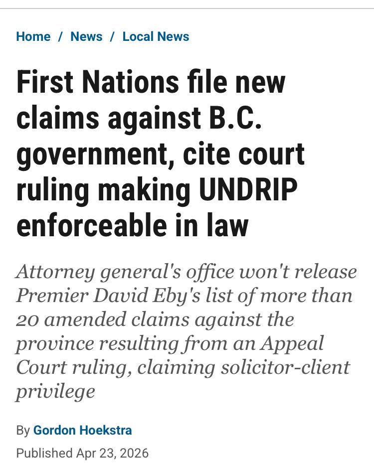
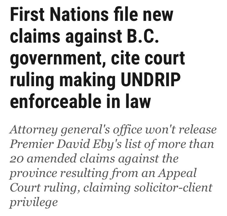
Apr 24
20 Cases and Counting.
The NDP Attorney General’s Grand Plan?
Negotiations with the FNLC in the ‘hope’ of ‘trying’ to find a solution to this legal mess.
Not Good Enough.
Why won’t the NDP make a decision and suspend/amend DRIPA which they KNOW needs to happen?
1️⃣The AG and Premier don’t want FN protests on their watch and will avoid the bad PR at all costs.
2️⃣The NDP values their relationship with the FNLC more than legally protecting 5.7 million British Columbians from endless litigation.
This is a complete loss of control by the NDP and they should dissolve this parliament and call an election.
Let the people decide who they actually want to lead us out of this chaos.
#bcpoli
1
12
519