
Mar 16
PostgresTV: Regina Obe and Paul Ramsey to discuss PostGIS youtube.com/watch?v=JDULwjz1…

7
663

23 Dec 2025
PostgresTV hacking session live — join! we dig into direction of support of btree merge again (because now it has only split, hence inevitable index bloat and need to rebuild index), a hard but super interesting topic youtube.com/watch?v=c0wKWcPZ…
1
4
1,393
7 Feb 2024
The proposed UUIDv7 support in @PostgreSQL that was started during a #PostgresTV session with Kirk, Andrey @x4mmmmmm and myself (youtube.com/live/YPq_hiOE-N8…) received attention and was on HN frontpage yesterday: news.ycombinator.com/item?id… -- interesting to read a wider range of opinions
1
8
53
3,706

21 Nov 2023
1. @hnasr
2. @thegeeknarrator
3. @vaibhaw_vipul
4. Anthony Writes Code
5. Ritvikmath
6. Jon Gjengset
7. Low Byte Productions
8. CMU Database Group
9. Anthony GG
10. Tsoding
11. PostgresTV
12. Ben Langmead
13. Code Aesthetic
14. Nanobyte
15. Dmitry Soshnikov
16. Jacob Sorber
17. David Beazley
And a bunch of conference channels.
These are some I follow. There are many more which I have not yet come across. I typically find an interesting channel and go through every single video from it that I find interesting.
And then I switch to another one.
6
6
67
4,563
8 Oct 2023
#PostgresMarathon day 12: How to find query examples for problematic pg_stat_statements records
// I post a new @PostgreSQL "howto" article every day. Join me in this journey – subscribe, provide feedback, share!
In a few hours, I'm making my "Seamless Postgres query optimization" tutorial at @djangocon, so it's a good time to talk about transitioning from pg_stat_statements (pgss) to EXPLAIN.
## The problem of jumping from pgss to EXPLAIN
Once a problematic pgss record is identified (which is the subject of query macro-optimization that we've discussed on days 5-7 twitter.com/samokhvalov/stat…), the first thing to do is to understand the direction of optimization.
Two most common basic situations of pgss records requiring optimization:
1. If "calls" is very high (a lot of QPS, queries per second), the main method to optimize is reduction of this number – this is to be done on client (app) side.
2. If "mean_exec_time mean_plan_time" is high (for the OLTP context – web and mobile apps – 100ms should be considered slow: postgres.ai/blog/20210909-wh…), this is when we need to apply query micro-optimization – use EXPLAIN.
Of course, it's also not uncommon to have a combination of these two basic cases – quite frequent query with poor latency.
In this post, we won't discuss how to use EXPLAIN and EXPLAIN (ANALYZE, BUFFERS). Instead, we'll focus on finding proper materials for EXPLAIN – particular query examples that need to be studied and improved.
It is worth remembering that a single pgss records can be associated with individual queries that are executed differently – using different plans. A basic example illustrating it:
nik=# create table t1 as select 1::int8 as c1;
SELECT 1
nik=# insert into t1 select 2
from generate_series(1, 1000000);
INSERT 0 1000000
nik=# create index on t1(c1);
CREATE INDEX
nik=# vacuum analyze t1;
VACUUM
nik=# explain select from t1 where c1 = 1;
QUERY PLAN
-------------------------------------------------------------------------
Index Only Scan using t1_c1_idx on t1 (cost=0.42..4.44 rows=1 width=0)
Index Cond: (c1 = 1)
(2 rows)
nik=# explain select from t1 where c1 = 2;
QUERY PLAN
------------------------------------------------------------
Seq Scan on t1 (cost=0.00..16981.01 rows=1000001 width=0)
Filter: (c1 = 2)
(2 rows)
– both queries here will be registered as "select * from t1 where c1 = $1" in pgss. But plans are different, because for "c1 = 1", we have high selectivity, while for "c1 = 2" it is really bad (targeting all but 1 rows in the table).
This means that looking at just pgss record demonstrating poor query latency, we cannot quickly jump to using EXPLAIN – we need to find particular query samples to work with.
Below, we discuss options to solve this problem.
## Option 1: guessing
In some cases, it may be fine to guess. But, I had really bad cases when I lost a lot of time making a mistake with guessing. For example, in one case, dealing with a boolean column, I decided to use the value that had a very bad selectivity, and spent a lot of time optimizing this situation, before realizing that application code never ever is going to use it.
It might be tempting to use pg_statistic to improve the guesswork. But unfortunately, in general case, this doesn't work really well, because of lack of multi-column statistic (except when it's created explicitly) – without it, we're going to have unrealistic parameter variants in lots of cases.
So this method is limited and can be used only for simple cases.
## Option 2: get examples from Postgres log
It is possible to find examples in the Postgres log – of course, if they are logged (usually via the log_min_duration_statement parameter or the auto_explain extension). To find examples for a given pgss record, we need to be able to find association of logged queries and pgss records. Two options:
1. For PG14 , option compute_query_id (postgresqlco.nf/doc/en/param…) can provide the same queryid value that is used in pg_stat_statements, to the log entry.
2. Alternatively, we can use an excellent library libpg_query (github.com/pganalyze/libpg_q…; Ruby, Go, Python and other options are also available). It can be applied both to normalized (pgss records) and individual queries, producing so-called fingerprint, that can be then used to find the relationships we need.
In general, using Postgres logs to find query examples is a good method, but for heavily-loaded systems, where it is impossible to log all queries, it is going to supply us with very slow examples only – those that exceed log_min_duration_statatement postgresqlco.nf/doc/en/param…(usually set to some quite high value, e.g. 500ms).
This situation can be improved with sampling and lowering the threshold for slow queries or even getting rid of it completely. Parameters for it:
- log_min_duration_sample (PG13 ) postgresqlco.nf/doc/en/param…
- log_statement_sample_rate (PG13 ) postgresqlco.nf/doc/en/param…
- postgresqlco.nf/doc/en/param… (PG12 ) postgresqlco.nf/doc/en/param…
Alternatively, auto_explain can be used, it also supports sampling (auto_explain.sample_rate, all currently supported versions), and it can look really attractive since it brings plans as they were right on production. Installation of auto_explain should be done with careful testing and analysis of overhead.
## Option 3: sample queries from pg_stat_activity
This method can be attractive since it doesn't require us to turn on the expensive logging of too many queries. And even low-latency queries, if they are frequent enough, are going to be eventually captured if we observe pg_stat_activity.query long enough.
However, there are two important limitations here.
First, the column pg_stat_statements.query_id, useful to connect samples from pg_stat_activity (pgsa) with pgss records, was added relatively recently, in PG14. For older versions, we would end up using some regular expressions (implementation can be cumbersome/fragile) of libpg_query's fingerprints (meaning that we need to sample all pgsa records and then post-process them). So this method is better to use in PG14 .
Second, by default, pg_stat_activity.query is truncated to 1024 characters – this is defined by track_activity_query_size (track_activity_query_size), which is 1024 by default. It is recommended to increase it significantly – e.g., to 10k, to allow larger queries to be sampled and analyzed. Unfortunately, changing this setting requires a restart.
## Option 4: eBPF
This option is not yet fully developed, but there is an opinion that it can be a very good alternative in the future: use eBPF for either sampling queries (alternative to pgsa), or even for sampling queries normalizing them (being alternative to both pgsa pgss).
So – TBD. Meanwhile, check out these interesting resources:
- pgtracer github.com/Aiven-Open/pgtrac… (presentation on PostgresTV: youtube.com/watch?v=tvJgMV-8…)
- Analyzing Postgres performance problems using perf and eBPF – a talk video where Andres Freund describes how to combine pg_stat_statements BPF youtu.be/HghP4D72Noc?si=tFuQ… (code: github.com/anarazel/pg-bpftr…)
## Summary
- In PG14 , use compute_query_id to have query_id values both in Postgres logs and pg_stat_activity
- Increase track_activity_query_size (requires restart) to be able to track larger queries in pg_stat_activity
- Organize workflow to combine records from pg_stat_statements and query examples from logs and pg_stat_activity, so when it comes to query optimization, you have good examples ready to be used with EXPLAIN (ANALYZE, BUFFERS).
As a reminder, once you have good examples, the best (fastest&cheapest) way to verify optimization ideas is to use properly tuned thin clones – check out DBLab @Database_Lab.
---
3 Oct 2023

#PostgresMarathon, day 7: How to work with pg_stat_statements, part 3
Previous parts:
- part 1: twitter.com/samokhvalov/stat…
- part 2: twitter.com/samokhvalov/stat…
3rd type of derived metrics: percentage
Now, let's examine the third type of derived metrics: the percentage that a considered query group (normalized query or bigger groups such as "all statements from particular user" or "all UPDATE statements") takes in the whole workload with respect to metric M.
How to calculate it: first, apply time-based differentiation to all considered groups (as discussed in the part 1 twitter.com/samokhvalov/stat…) — dM/dt — and then divide the value for particular group by the sum of values for all groups.
Visualization and interpretation of %M
While dM/dt gives us absolute values such as calls/sec or GiB/sec, the %M values are relative metrics. These values help us identify the "major players" in our workload considering various aspects of it — frequency, timing, IO operations, and so forth.
Analysis of relative values helps understand how big is the potential win from each optimization vector and prioritize our optimization activities, first focusing on those having the most potential. For example:
- If the absolute value on QPS seems to be high — say, 1000 calls/sec — but if it represents just 3% of the whole workload, an attempt to reduce this query won't give a big win, and if we are concerned about QPS, we need to optimize other query groups.
- However, if we have 1000 calls/sec and see that it's 50% of the whole, this single optimization step — say, reducing it to 10 calls/sec — helps us shave off almost half of all the QPS we have.
One of the ways to deal with proportion values in larger systems is to react on large percentage values, consider the corresponding query groups as candidates for optimization. For example, in systems with large number of query groups, it might make sense to apply the following approach:
- Periodically, for certain metrics (for example, "calls", "total_exec_time", "total_plan_time", "shared_blks_dirtied", "wal_bytes"), build top-10 lists showing query groups having the largest %M values.
- If particular query group turns out to be a major contributor – say, >20% — on certain metrics, consider this query as a candidate for optimization. For example, in most cases, we don't want a single query group to be responsible for 1/2 of the aggregated total_exec_time ("total total_exec_time", apologies for tautology).
– In certain cases, it is ok to decide that query doesn't require optimization — in this case we mark such group as exclusion and skip it in the next analyses.
The analysis of proportions can also be performed implicitly, visually in monitoring system: observing graphs of dM/dt (e.g., QPS, block hits per second), we can visually understand which query group contributes the most in the whole workload, considering a particular metric M. However, for this, graphs need to be "stacked" en.wikipedia.org/wiki/Bar_ch….
If we deal with 2 snapshots, then it makes sense to obtain such values explicitly. Additionally, for visualization purposes, it makes sense to draw a pie chart for each metric we are analyzing.
%M examples
1. %M, where M is "calls" — this gives us proportions of QPS. For example, if we normally have ~10k QPS, but if some query group is responsible for ~7k QPS, this might be considered as abnormal, requiring optimizations on client side (usually, application code).
2. %M, where M is "total_plan_time total_exec_time" — percentage in time that the server spends to process queries in a particular group. For example, if the absolute value is 20 seconds/second (quite a loaded system — each second Postgres needs to spend 20 seconds to process queries), and a particular group has 75% on this metric, it means we need to focus on optimizing this particular query group. Ways to optimize:
- if QPS (calls/second) is high, then, first of all, we need to reduce
- if average latency (total_exec_time, less often total_plan_time or both) is high, then we need to apply micro-optimization using EXPLAIN and EXPLAIN (ANALYZE, BUFFERS).
- in some cases, we need to combine both directions of optimization
3. %M, where M is "shared_blks_dirtied" — percentage of changes in the buffer pool performed by the considered query group. This analysis may help us identify the write-intensive parts of the workload and find opportunities to reduce the volume of checkpoints and amount of disk IO.
4. %M, where M is "wal_bytes" — percentage of bytes written to WAL. This helps us identify those query groups where optimization will be more impactful in reducing the WAL volumes being produced.
Instead of summary: three macro-optimization goals and what to use for them
Now, with the analysis methods described here and in the previous 2 parts, let's consider three popular types of macro-optimization with respect to just a single metric — total_exec_time.
Understanding each of these three approaches (and then applying this logic to other metrics as well) can help you understand how your monitoring dashboards should appear.
1. Macro-optimization aimed to reduce resource consumption. Here we want to reduce, first of all, CPU utilization, memory and disk IO operations. For that, we need to use the "dM/dt" type of derived metric – the number of seconds Postgres spends each second to process the queries. Reducing this metric — the aggregated "total" value of it for the whole server, and for the Top-N groups playing the biggest role — has to be our goal. Additionally, we may want to consider other metrics such as shared_blks_***, but the timing is probably the best starting point. This kind of optimization can help us with capacity planning, infrastructure cost optimization, reducing risks of resource saturation.
2. Macro-optimization aimed to improve user experience. Here we want our users to have the best experience, therefore, in the OLTP context, we should focus on average latencies with a goal to reduce them. Therefore, we are going to use "dM/dc" — number of seconds (or milliseconds) each query lasts on average. If in the previous type of optimization, we would like to see Top-N query groups ordered by the "dM/dt" values (measured in seconds/second) in our monitoring system, here we want Top-N ordered by avg. latency (measured in seconds). Usually, this gives us a very different set of queries — perhaps, having lower QPS. But these very queries have worst latencies and these very queries annoy our users the most. In some cases, in this this type of analysis, we might want to exclude query groups with low QPS (e.g., those having QPS < 1 call/sec) or exclude specific parts of workload such as data dump activities that have inevitably long latencies.
3. Macro-optimization aimed to balance workload. This is less common type of optimization, but this is exactly where %M plays its role. Developing our application, we might want, from time to time, check Top-N percentage on total_exec_time total_plan_time and identify query groups holding the biggest portion — exactly as we discussed above.
Bonus: podcast episodes
Related @PostgresFM episodes::
- Intro to query optimization postgres.fm/episodes/intro-t…
- 102 query optimization postgres.fm/episodes/102-que…
- pg_stat_statements postgres.fm/episodes/pg_stat…
---
That concludes our discussion on pgss for now. Of course, this was not a complete guide, we might return to this important extension in the future.
Let me know if you have questions or any other feedback!
2
5
59
10,495
29 Aug 2023
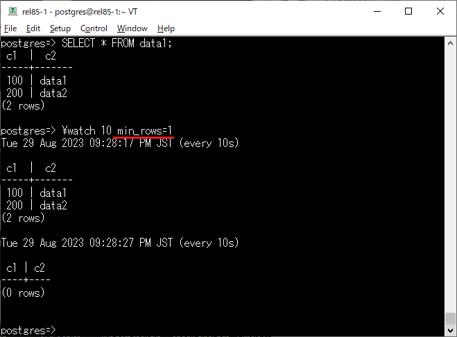
I'm happy to see this.
I always lacked the ability to stop execution of \watch loops in psql. Proposed this idea for our live coding on #PostgresTV, @x4mmmmmm implemented (youtube.com/live/vTV8XhWf3mo…), it was committed to PG16.
The implementation was flexible -- any option is possible to add later. And here we see it, for PG17 🆒👍
29 Aug 2023

PostgreSQL 17 dev: Allow \watch queries to stop on minimum rows returned
git.postgresql.org/gitweb/?p…
1
1
11
1,923

28 Aug 2023
We had an amazing chat with @samokhvalov from @PostgresFM & #PostgresTV on why @ferret_db uses @postgreSQL and how we are building an #opensource #database alternative to #MongoDB
Watch the episode here --> buff.ly/3svTOa0
1
9
575
22 Jun 2023
Again, a wave of interest to the performance issues of traditional UUID with a post by @PostgresSupport and HN discussion: news.ycombinator.com/item?id…
We discussed some of these problems here during a #PostgresTV session, and developed a patch to support ULID / UUIDv7: youtube.com/watch?v=YPq_hiOE…
And then Andrey proposed a patch in -hackers: postgresql.org/message-id/fl…
Everyone who can help (test, discuss, etc.) – please participate in that discussion.
5
12
7,726
26 May 2023
New feature in PG16 psql:
\watch i=1 c=3
This is probably the first @PostgreSQL feature that was implemented online – during #PostgresTV stream with @x4mmmmmm: youtube.com/watch?v=vTV8XhWf…

8
1,188
4 May 2023
In ~30 min we'll have a #PostgresTV online session with @ahachete and @michristofides to discuss open source licenses in Postgres ecosystem youtube.com/live/1rcbyIjA4gI - join!
And right after that - a Hacking session with @x4mmmmmm and Kirk, as usual.
2
6
877

In this recent @PostgresTV episode, @Samokhvalov interviews Percona Founder @PeterZaitsev about his take on #PostgreSQL and its biggest problems compared to any other #database.
Tune in to watch the full episode here 👇 bit.ly/3mjsYyA
3
4
702

6 Mar 2023
Watch a new interview with @PeterZaitsev in #PostgresTV:
youtube.com/watch?v=curz6Tx8…
#PostgreSQL #opensource #databases #Percona
1
3
398
23 Feb 2023
#PostgresTV @PostgreSQL Hacking 101 live session with Andrey and Kirk: youtube.com/watch?v=RiROxnPi…
Join live for fun (chat is open) or watch it recorded later 🙂
1
2
766
11 Feb 2023
A patch developed by @x4mmmmmm during our #PostgresTV session this week has just been sent to -hackers: postgresql.org/message-id/CA…
1/3
2
16
1,515
9 Feb 2023
We're going to create another small patch, fast ULID – youtube.com/watch?v=YPq_hiOE… #PostgresTV
(apologies for short notice)
it's online right now -- join
2
2
17
3,200

29 Jan 2023
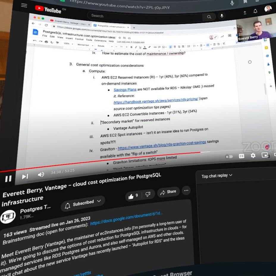
Great infos for cloud cost optimization in #PostgresTV with @retttx (@joinvantage) and @samokhvalov
youtu.be/ZPL-j0pJPiY
1
2
15
1,751

26 Jan 2023
#PostgresTV tomorrow (Jan 26) at 9am PT / 12pm ET / 16:00 UTC – with Everett Berry @retttx (@JoinVantage)
The topic is of growing importance:
@PostgreSQL infrastructure cost optimization – with a focus on clouds, RDS, etc.
Join live 💙 or watch later: youtube.com/watch?v=ZPL-j0pJ…
1
11
615
5 Jan 2023
#PostgresTv session with the cofounders of Hydra @HydrasDB ("open source Snowflake") moved to Monday – apologies, there was a coordination issue from my side, it happens sometimes.
But on Monday (Jan 9), at 9am PT (17:00 UTC), we'll do it: youtube.com/watch?v=71eD53lt… - don't miss.
1
5
1,210
15 Dec 2022
Missed it, will watch it later. You can learn a lot on troubleshooting performance on Linux systems from @erthalion on #postgrestv
15 Dec 2022
The hardcorest talk ever presented on Postgres.tv 😅
I need to rewatch it with notebook and pen for notes.
Do I have followers who don't see anything new in it⁉️
1
9
915
24 Oct 2022
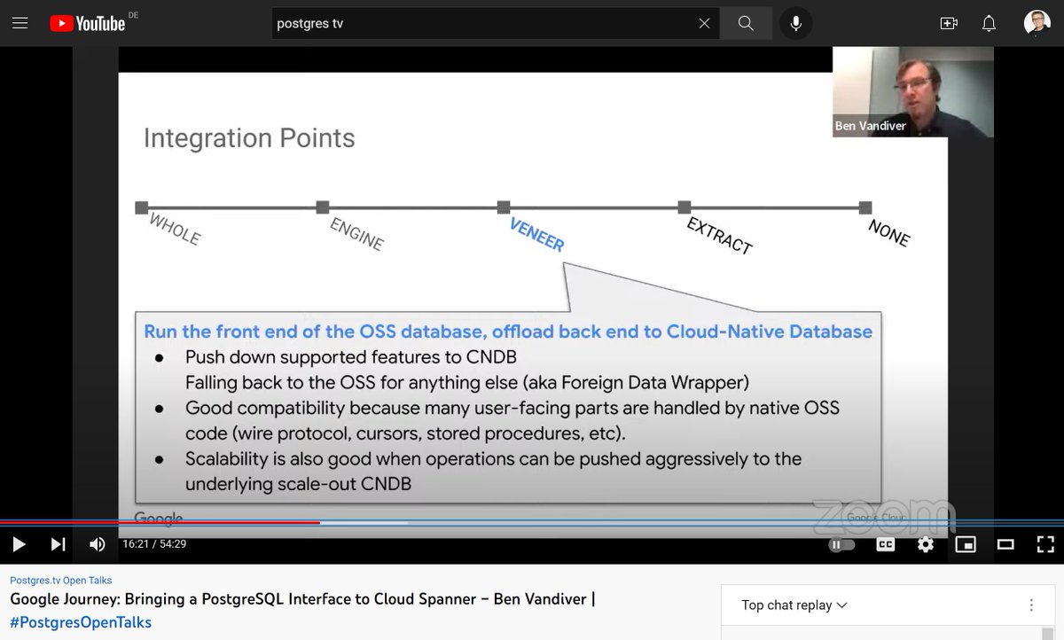
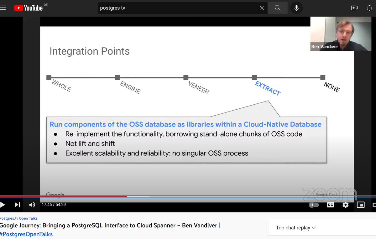
Another great #postgrestv episode, with @benvandiver about postgres-compatibility in @Google Spanner
youtube.com/watch?v=BW-Uexhv…
🤔@YugabyteDB is in the “VENEER” category (using PG for the query layer) where #spanner “EXTRACT”s limited code without the goal of lift&shift from/to PG
19 Oct 2022

"Google Journey: Bringing a @PostgreSQL Interface to Cloud Spanner" will be presented by Ben Vandiver this Thursday at the usual time, 17:00 UTC / 1pm ET / 10am PT
#PostgresOpenTalks
youtu.be/BW-Uexhv-bk
1
6