
Imagine a drunk man staggering along a cliff. Each step he takes is random—will he fall off?
This is the essence of 1-D random walks! Understanding these concepts not only deepens your appreciation for probability but also enhances your skills in quantitative research. Let’s explore the fascinating world of randomness together!
#RandomWalks #QuantResearch #Probability #DataScience #MyntBit #MathFun

13

Jun 11
decomposition of anomalous diffusion in two-state #randomwalks.
flashontrack.blogspot.com/20…
7

ich habe Mathematik mit Schwerpunkt Wahrscheinlichkeitsrechnung, RandomWalks und Statistik studiert und Biologie auf Diplom fast komplett. Ich habe gelernt, wie man einen Test konstruiert, um Risiken abzusichern.
Je schlimmer das Ereignis ist, umso grösser darf der Aufwand sein.
6
2
44

Mar 20
Kiyosi Itô and the Birth of Stochastic Calculus
Once you swallow the fact that Brownian motion is continuous everywhere and differentiable nowhere, Itô’s quadratic variation is the next quiet shock waiting for you.
Ordinary smooth curves have zero quadratic variation. If you chop time into tiny pieces and add up (increment)² over the interval, that sum goes to zero as your partition gets finer. But for Brownian motion that same sum doesn’t vanish, it locks onto the length of the time interval.
So, you have this path with no velocity anywhere, but its squared wiggles accumulate in a completely rigid, deterministic way. Over time T, the total quadratic variation is exactly T.
So, you lose the classical derivative, but you gain a new calculus where the (dB)² term behaves like dt, and suddenly integrals against Brownian motion make sense and you can do Stochastic Calculus.
Brownian motion refuses to be smooth, but its roughness is so structured that when you look at it through the lens of quadratic variation, the randomness averages out and you’re left with a clean clock ticking underneath the noise.
#BrownianMotion #ProbabilityTheory #StochasticCalculus #RandomWalks #Ito #QuadraticVariation
7
20
144
7,460
Mar 20
The Curve That Forced Japanese Mathematician Kiyosi Itô to Invent A New Calculus
A Brownian path is a strange object. It traces a continuous curve without ever jumping, yet at no point does it settle into a well-defined direction, so it is continuous everywhere but differentiable nowhere!
No matter how much we magnify, the path won’t straighten out. It keeps wrinkling at every scale.
#BrownianMotion #StochasticProcesses #RandomWalks #ProbabilityTheory
7
27
235
16,305
Feb 10
The more you study 20th-century Probability Theory, the more you see how the Russian School trained a certain kind of engineering mind.
When you hear about modern high-end systems coming out of that ecosystem, including nuclear energy, space and hypersonic missile programs, it doesn’t feel like it came from nowhere.
Giants of the Russian School of Probability Theory Turned Noise into Structure.
In 1906, Andrey A. Markov asked what sounded like a heretical question at the time. If randomness is allowed to remember something, even just the present, does probability theory fall apart?
His answer was surprisingly calm. You let the next step depend only on where you are now,
P(Xₙ₊₁ = j | Xₙ = i, Xₙ₋₁, …) = Pᵢⱼ,
and nothing collapses. Individual paths stay noisy, but long-run averages still behave. State frequencies settle down to a fixed profile π with
π = πP.
The bead jitters forever, but the glow it leaves behind stabilizes.
That idea turned out to be everywhere. Random-walk estimates. MCMC, where you build a chain whose stationary distribution is the thing you want and then trust time averages. Hidden Markov models in time series. Ion channels flicking open and shut. Control and reinforcement learning, where the world resets its memory at every step. One simple constraint, enormous reach.
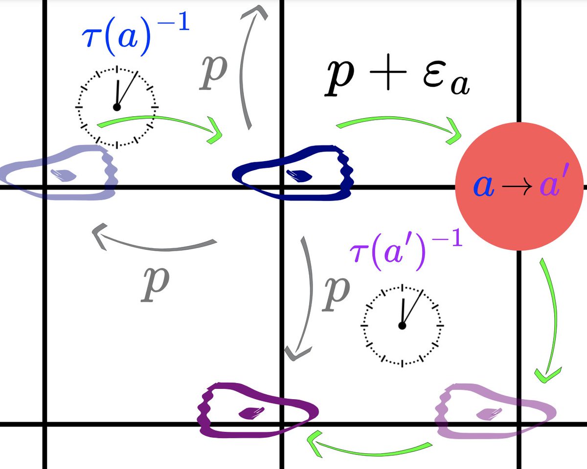
Then, in 1931, Andrey Nikolaevich Kolmogorov took Markov’s step-by-step idea and tilted it sideways. Instead of only asking where the chain spends its time in the long run, he asked how the entire distribution moves right now.
In continuous time, the same Markov mechanism becomes dynamics:
dp/dt = pQ,
with Q the generator. Probability stops being a static histogram and turns into something that flows. In the render, that’s the fog spreading through the maze. The flux layer is the net current pushed through corridors and the portal. The particles are just sample paths of the same generator. One process, three ways of seeing it.
The final shift is more subtle. If the forward equation tells you how probability moves, there’s another question it doesn’t answer on its own. From a given state, what does the future look like?
Pick two terminal sets, A and B, and define
q(x) = Pₓ[hit B before A].
That q isn’t a density. It’s a forecast attached to each state. Kolmogorov’s backward view says this forecast is harmonic in the interior. With boundary conditions q = 0 on A and q = 1 on B, it satisfies
Lq = 0.
Now the background field in the render isn’t where probability is. It’s how likely success is. Dark regions mean you’re probably doomed to hit A first. Bright regions mean B is likely. The sharp transition near the portal is where the decision really gets made.
Over that chance map, the forward fog starts moving. Probability mass bunches in narrow corridors, spills around corners, and streams through the portal. The glowing filaments show the dominant routes toward B. The particles just trace those same routes as individual random paths.
All three views come from the same Markov generator. Long-run averages. Time-evolving distributions. State-by-state forecasts. Same mechanism, different lenses.
#ProbabilityTheory #MarkovChains #Kolmogorov #StochasticProcesses #MCMC #RandomWalks #BackwardEquation #ForwardEquation #AppliedProbability #Mathematics #Russian #Russians
17
45
311
13,998
Feb 7
Once you accept that a Brownian path is continuous everywhere and differentiable nowhere, the next quiet shock is Itô’s quadratic variation.
For an ordinary smooth curve, the story is boring. Chop time into tiny pieces, add up (increment)² across the interval, and as you refine the partition that sum goes to zero.
Brownian motion does the opposite. Do the same thing and the sum doesn’t vanish. It settles down. Over an interval of length T, the total quadratic variation comes out to exactly T.
So you end up with a path that has no velocity anywhere, but whose squared wiggles add up in a rigid, deterministic way.
So, you give up the classical derivative, and you get a new calculus where the dB·dB term behaves like dt. Then integrals against Brownian motion stop being nonsense and the so-called Stochastic Calculus becomes a real thing.
#BrownianMotion #ProbabilityTheory #StochasticCalculus #RandomWalks #Ito #QuadraticVariation
14
34
270
15,987
Feb 7
The Curve That Forced Mathematicians To Invent A New Calculus
There is a strange curve called Brownian path. It traces a continuous path without ever jumping, but it never settles into a well-defined direction at any point, so it’s continuous everywhere but differentiable nowhere.
We’re used to the idea that if something is continuous, then if you zoom in far enough it should start to look like a straight line. A Brownian path refuses. Zoom in and you don’t reveal a hidden tangent. You reveal fresh roughness.
This animation is a microscope on that fact. No matter how much we magnify, the path won’t straighten out. It keeps wrinkling at every scale.
#BrownianMotion #StochasticProcesses #RandomWalks #ProbabilityTheory #Fractals #MathAnimation
28
45
381
31,692
21 Dec 2025
Once you swallow the fact that Brownian motion is continuous everywhere and differentiable nowhere, Itô’s quadratic variation is the next quiet shock waiting for you:
Ordinary smooth curves have zero quadratic variation...if you chop time into tiny pieces and add up (increment)² over the interval, that sum goes to zero as your partition gets finer. But for Brownian motion that same sum doesn’t vanish, it locks onto the length of the time interval.😲
So, you have this path with no velocity anywhere, but its squared wiggles accumulate in a completely rigid, deterministic way. Over time T, the total quadratic variation is exactly T. 🫡
That’s the trade the universe makes here...you lose the classical derivative, but you gain a new calculus where the “dB times dB” term behaves like dt, and suddenly integrals against Brownian motion make sense and you can do stochastic calculus. 📝
Brownian motion refuses to be smooth, but its roughness is so structured that when you look at it through the lens of quadratic variation, the randomness averages out and you’re left with a clean clock ticking underneath the noise.
#BrownianMotion #ProbabilityTheory #StochasticCalculus #RandomWalks #Ito #QuadraticVariation
41
69
701
100,531


5 Jul 2025
We only went and found an escaped #goat on our walkies tonight!! His back home where he belongs now 😂🤷🏼♀️😂 #randomwalks #walkies
6
109

11 Jun 2025
Scientists created an approximation for the return time distribution of #RandomWalks on undirected networks and tested it on many graphs, showing that local structure has a much larger influence than global structure.
Read the paper: go.aps.org/4mY8wye
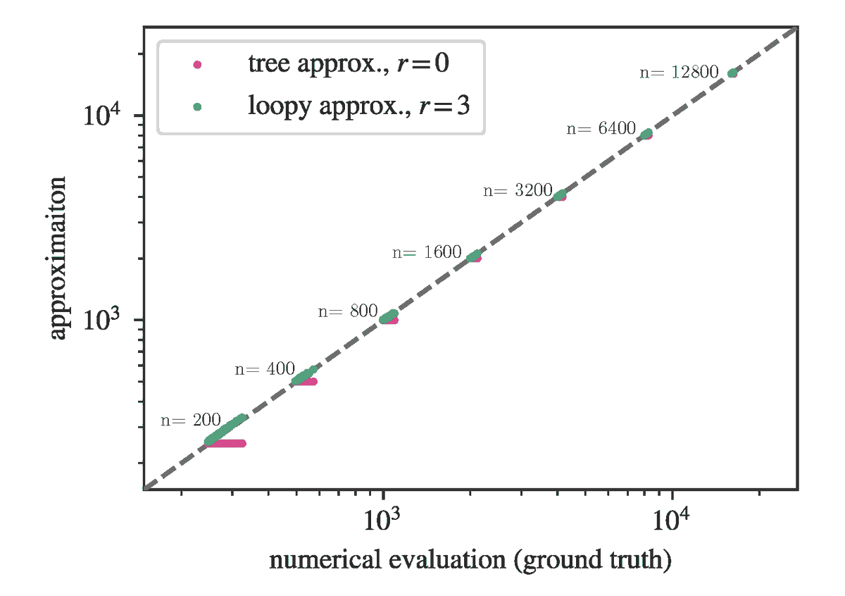
ALT Graph with “approximation” on the Y axis and “numerical evaluation (ground truth)” on the X axis. A diagonal dashed line bisects the graph at y=x. Tree approximations with r=0 are shown in red. When there are fewer nodes, the red approximations start moving toward the line, becoming more accurate. Green lines show loopy approximations with r=3. They are pretty accurate when there are few nodes.
1
5
15
813

29 May 2025
A drunk man will find his way home. A drunk bird may be lost forever. Searching, is one of the most important, yet underappreciated aspects of biology. #ComplexSystems #RandomWalks
28 May 2025

Probability of returning to the origin in a random walk:
1D → P=1
2D → P=1
3D → P=0.34
Large D → P=1/2D

3
274

27 Feb 2025
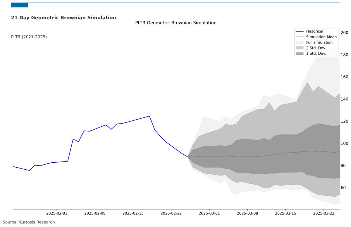
Taking a look at $PLTR wild ride. A little geometric brownian motion simulation has some thoughts about the next month. What do you think?
The model's half dozen parameters were tuned over the entirely of PLTR's history. every interval PLTR has been trading. Do #randomwalks, #montocarlo methods or #BrownianMotion (why are these not popular hash tags folks!? ) have a place in today's hype-driven markets?
Let's watch and find out. Ooh! It moves!
#Investing #palantir
8
4
1,119

22 Aug 2024
Imagine you’re at a big outdoor market looking for the best stall to buy fresh fruits.
Lévy Walks: You’re wandering around the market, making lots of quick, small stops at different stalls, checking out what’s available. Suddenly, you spot a stall way across the market that looks really promising, so you make a beeline for it, covering a lot of ground in one go.
Brownian Motion: Now that you’ve found a great stall, you stay in that area, slowly moving around to pick the best fruits from nearby stands. You’re not going far anymore—just sticking close and making small, deliberate moves to get what you want.
#ScienceExplained #RandomWalks #BehavioralScience #MathInNature #Physics #funtrivia
3
443

3 Jul 2024
Aging dynamics of 𝑑−dimensional locally activated random walks, Julien Brémont, Theresa Jakuszeit, R. Voituriez, and O. Bénichou #ActiveParticles #RandomWalks go.aps.org/3VTeiEu
8
34
1,344
3 May 2024
Extreme value statistics of jump processes, J. Klinger, R. Voituriez, and O. Bénichou #RandomWalks #ExtremeEvents go.aps.org/3wqrDeL
5
21
1,677

16 Apr 2024
🎬🆕ALEA Days
Tran, Viet Chi (2024). Random walks on simplicial complexes. CIRM. Audiovisual resource. dx.doi.org/10.24350/CIRM.V.2…
@_CIRM #Maths #conference #Probability #RandomWalks
1
2
30

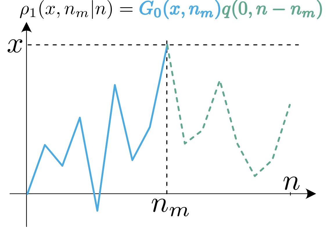
Great new work by Yanyang Wang, Wei Li, Feiyi Liu and Jianmin Shen at Central China Normal University and @ELTE_UNI - 'Supervised and unsupervised learning of (1 1)-dimensional...... #randomwalks' - iopscience.iop.org/article/1… #machinelearning #statphys #comphys #AI #neuralnetworks
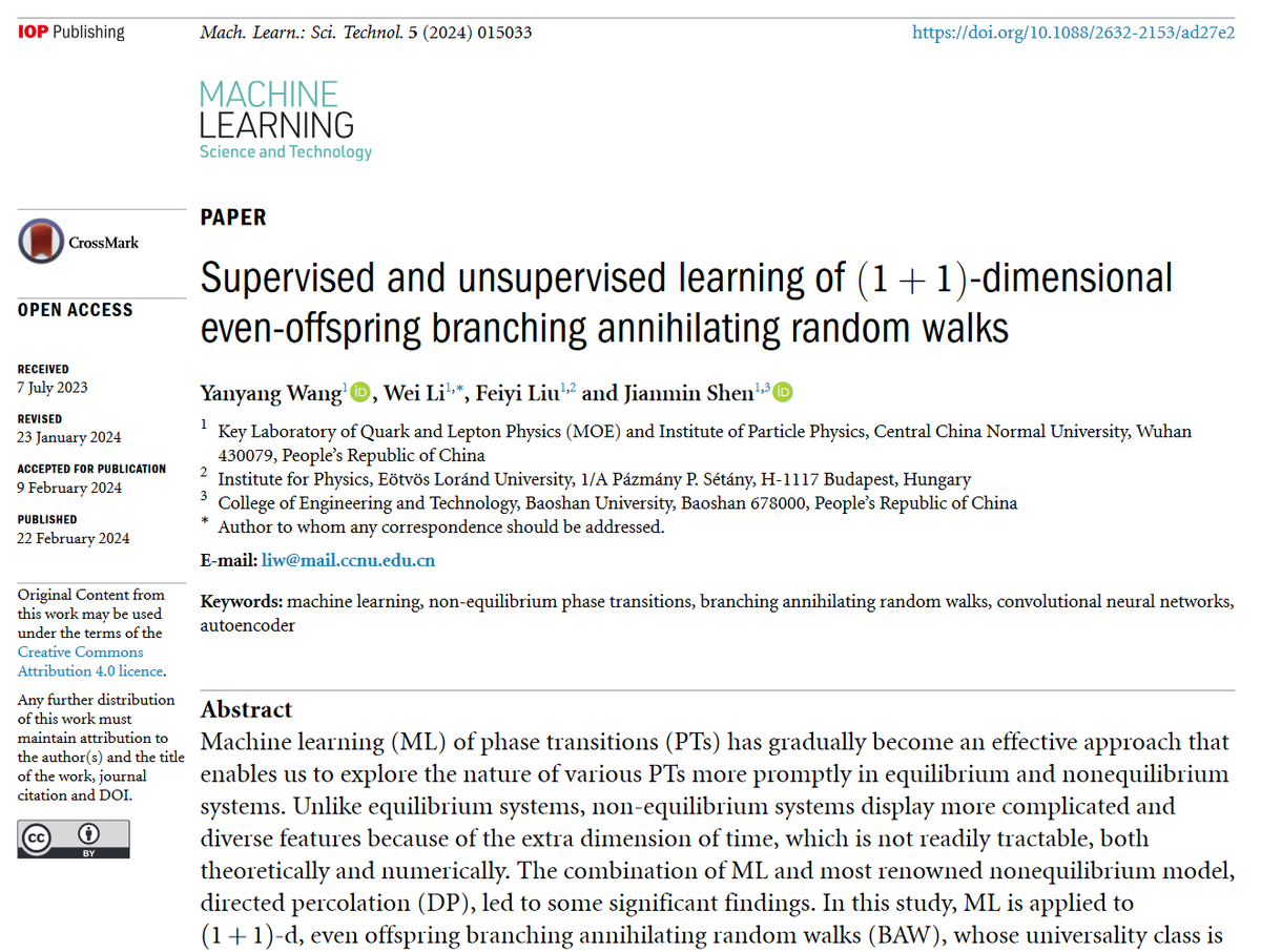
6
1,114