Use of Wolfram Mathematica for Neutrino Fourier Analysis Neutrino detection signals (e.g., from Cherenkov radiation in photomultiplier tubes or scintillation events) are inherently stochastic, sparse, and often embedded in substantial background noise. Fourier Transform (FT) methods enable decomposition of these time-domain signals into frequency-domain representations, facilitating identification of structure, periodicity, or characteristic spectral signatures. In Wolfram Mathematica, the core operation is the discrete Fourier transform (DFT), implemented via Fourier[list]. For a sampled signal s(tₙ) with uniform spacing Δt, Mathematica computes: S(ω_k) = Σₙ s(tₙ) exp(-2π i n k / N) where N is the number of samples. The corresponding frequency bins are obtained using FourierFrequencies[N, Δt]. Workflow: 1.Data ingestion Import detector time-series data (e.g., from IceCube-like event streams): data = Import[“neutrino_signal.dat”]; 2.Preprocessing Apply detrending and windowing to suppress spectral leakage: dataDetrended = data - Mean[data]; window = HannWindow[Length[data]]; dataWindowed = dataDetrended * window; 3.Fourier transform spectrum = Fourier[dataWindowed, FourierParameters -> {1, -1}]; 4.Power spectral density (PSD) psd = Abs[spectrum]^2; 5.Frequency axis freq = FourierFrequencies[Length[data], Δt]; 6.Visualization ListLinePlot[Transpose[{freq, psd}], PlotRange -> All] Key advantages for neutrino analysis: • Noise discrimination: Background noise (thermal, electronic) often exhibits broadband or known spectral profiles, while transient neutrino bursts may introduce localized excess power. • Burst detection: Short-duration neutrino events produce wide-band spectral signatures; clustering in frequency space can indicate structured emission. • Periodicity search: For astrophysical sources (e.g., pulsars, core-collapse supernova oscillations), periodic modulation may be detectable in the frequency domain. • Multi-scale analysis: Mathematica supports ShortTimeFourier and WaveletTransform, allowing time–frequency localization for non-stationary signals. Advanced extensions: • Filtering: filtered = InverseFourier[BandpassFilter[spectrum, {f₁, f₂}]]; • Cross-correlation (multi-detector coincidence): CrossCorrelation[data1, data2] • Spectral estimation improvements: Use WelchMethod or multitaper approaches (custom implementation) to reduce variance in PSD estimates. Limitations: • Sparse event statistics: Neutrino detections are often low-count, making classical FT assumptions (stationarity, dense sampling) imperfect. • Non-periodicity: Many neutrino signals are impulsive; FT spreads such signals across frequencies, reducing interpretability. • Detector response convolution: Observed signals are filtered by detector transfer functions, requiring deconvolution for physical interpretation. Conclusion: Mathematica provides a complete symbolic–numerical environment for implementing Fourier-based pipelines in neutrino physics. Its strength lies in rapid prototyping, exact control of transforms, and integration with higher-level analysis (statistical inference, symbolic modeling). For non-repetitive neutrino bursts, FT should be complemented with time–frequency methods to preserve transient structure.

wavelet transform is the new deep web in ml. everyone is talking about it, and it's about to shake the AI world to its core 🦞 #WaveletTransform #Solana �

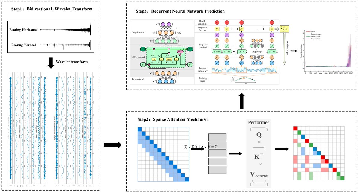
Check this newly published article "WaveAtten: A Symmetry-Aware #SparseAttention Framework for Non-Stationary Vibration #SignalProcessing" at brnw.ch/21wXpjo Authors: Xingyu Chen and Monan Wang #mdpisymmetry #wavelettransform #deeplearning

MTIWT(Moment Tensor using Wavelet Transform ): ✅ Simultaneous time/freq resolution ✅ Exact source params (mag/mech/depth) ✅ Robust for noisy/complex quakes Paper: doi.org/10.1007/s11600-025-0… #Seismology #Geophysics #MTIWT #WaveletTransform #SourceParams

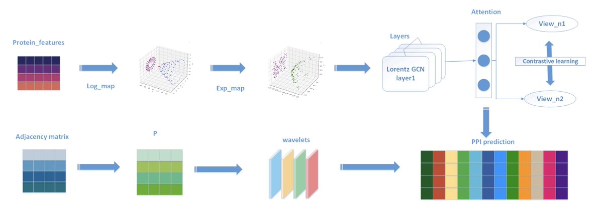
HyboWaveNet: Hyperbolic Graph Neural Networks with Multi-Scale Wavelet Transform for Protein-Protein Interaction Prediction 1. This paper introduces HyboWaveNet, a novel deep learning framework for protein–protein interaction (PPI) prediction that combines hyperbolic graph neural networks (HGNNs) with multi-scale graph wavelet transforms to capture complex biological hierarchies and dynamic interaction patterns. 2. HyboWaveNet maps protein nodes into Lorentz hyperbolic space, allowing the model to preserve and learn from the exponential, tree-like structure of protein interaction networks—structures that Euclidean GNNs struggle to represent without distortion. 3. The model applies LorentzGraphConvolution for neighborhood aggregation in hyperbolic space, leveraging exponential and logarithmic mappings to compute node embeddings that naturally reflect semantic distance and hierarchical topologies. 4. A key innovation is the use of random walk-based graph wavelet transforms to capture multiscale structural information. This allows the model to learn both local interactions (e.g., residue-level) and global modular structures (e.g., protein complexes). 5. HyboWaveNet includes a contrastive learning module that generates different augmented views of the same protein node and maximizes similarity between their embeddings, further enhancing the model’s generalization and robustness. 6. The model calculates interaction scores based on squared Lorentz distances between node embeddings, a biologically interpretable approach that reflects true hierarchical proximity in protein space. 7. On a benchmark PPI dataset from the HPRD database, HyboWaveNet achieves state-of-the-art performance with an AUC of 0.922 and an AUPR of 0.938, outperforming strong baselines like Struct2Graph, Fully HNN, and Topsy-Turvy. 8. Ablation studies confirm that removing either the hyperbolic encoder or the wavelet transform module significantly degrades model performance, highlighting the necessity of both geometry-aware learning and multiscale signal extraction. 9. Hyperparameter sensitivity analysis reveals optimal performance at 3–4 wavelet scales, aligning well with the biological intuition of hierarchical PPI networks that span local to global resolutions. 10. By combining geometric deep learning with signal processing, HyboWaveNet offers a powerful, interpretable, and biologically aligned solution for modeling protein–protein interactions—an essential step for drug target discovery and systems biology. 💻Code: github.com/chromaprim/Hybowa… 📜Paper: arxiv.org/abs/2504.20102 #PPI #GraphNeuralNetworks #HyperbolicGeometry #WaveletTransform #ProteinInteraction #AI4Science #ComputationalBiology #Bioinformatics

Multibranch Wavelet-Based Network for Image Demoiréing mdpi.com/1424-8220/24/9/2762 #wavelettransform #deeplearning #imagerestoration

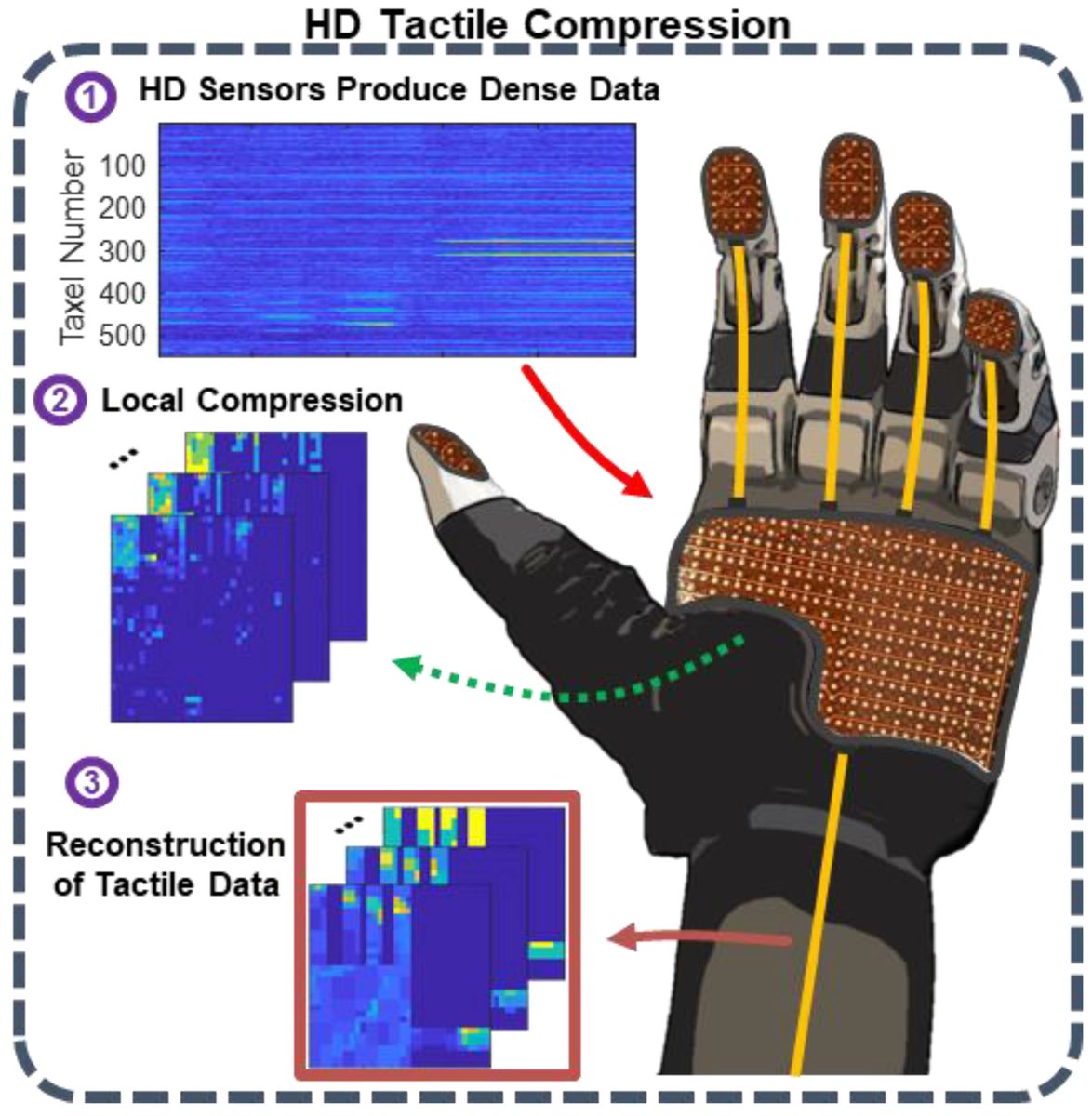
Wavelet Transforms Significantly Sparsify and Compress Tactile Interactions mdpi.com/1424-8220/24/13/424… @JohnsHopkins #spatiotemporal; #tactilesensing; #wavelettransform

Derivative-based wavelet transforms enhance structural damage detection with high accuracy, refining fault detection in engineering applications. Learn more: [link.springer.com/article/10…] #StructuralEngineering #WaveletTransform #DamageDetection #EngineeringResearch

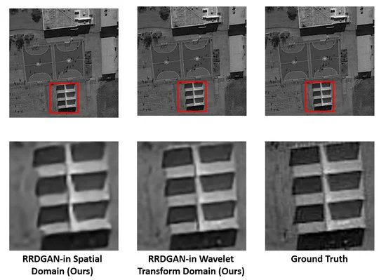
#mostcited 📢 #OpticalRemoteSensing #ImageDenoising and Super-Resolution #Reconstructing Using Optimized #GenerativeNetwork in #WaveletTransform Domain by Xubin Feng, Wuxia Zhang, Xiuqin Su and Zhengpu Xu 🔗 Read the full article: mdpi.com/2072-4292/13/9/1858

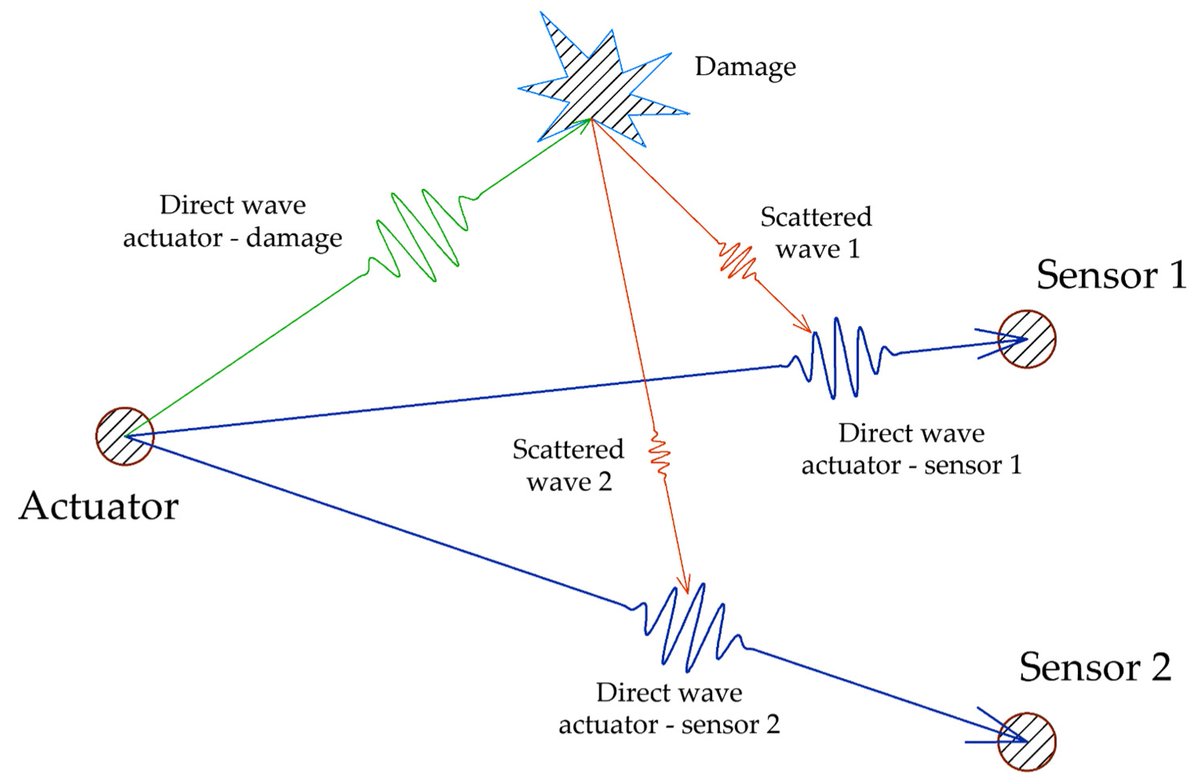
#highlycitedpaper Damage Localization in Composite Plates Using Wavelet Transform and 2-D #ConvolutionalNeuralNetworks mdpi.com/1424-8220/21/17/582… #ultrasonicguidedwaves #structuralhealthmonitoring #machinelearning #wavelettransform #damageimaging

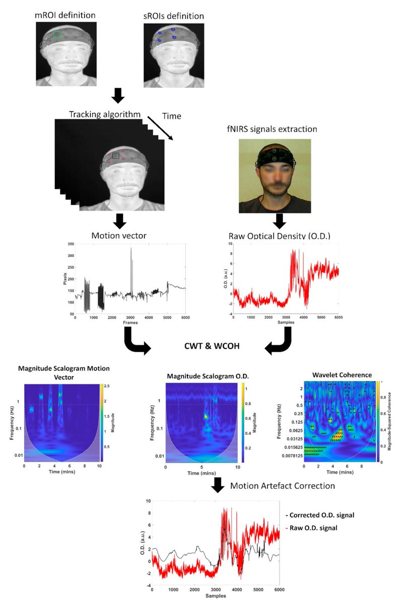
#highlycitedpaper A Motion Artifact Correction Procedure for fNIRS Signals Based on Wavelet Transform and Infrared Thermography Video Tracking mdpi.com/1424-8220/21/15/511… @univUda #motionartefacts #fNIRS #infraredimaging #infraredthermography #wavelettransform #trackingalgorithms

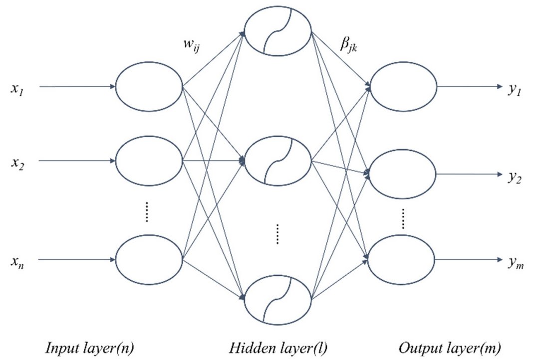
#mdpientropy #topcitedpaper: "A Hybrid Method Based on Extreme Learning Machine and Wavelet Transform Denoising for Stock Prediction". See more details at: mdpi.com/1099-4300/23/4/440. #stockprediction #extremelearningmachine #wavelettransform #deeplearning

On demand now: Fault Diagnosis in Smart Grid webinar. bit.ly/Dhend-replay This webinar covers topics of fault diagnosis, how it is done, and more. Stream it today. #IEEESmartGrid #faultdiagnosis #wavelettransform

On demand now: Fault Diagnosis in Smart Grid webinar. bit.ly/Dhend-replay This webinar covers topics of fault diagnosis, how it is done, and more. Stream it today. #IEEESmartGrid #faultdiagnosis #wavelettransform

Interested in learning about the basics of fault diagnosis in smart grid, including wavelet transform applications? bit.ly/Dhend-live Register now for this webinar on Fault Diagnosis in Smart Grid. @ieee_pes #IEEESmartGrid #faultdiagnosis #wavelettransform

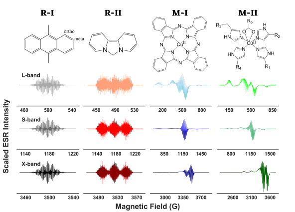
📢Read new paper on topic "ESR Spectra" by Aritro Sinha Roy and Madhur Srivastava @Cornell #openaccess @MDPIOpenAccess 👉 mdpi.com/2312-7481/8/3/32 #hyperfinedecoupling #ESR #resolutionenhancement #wavelettransform #signalprocessing

New #SpecialIssue "Wavelet Analysis for Data Science", edited by Dr. Dimitrios Tsoumakos and Dr. Ioannis Mytilinis, deadline 31 March 2022. Look forward to your submissions! mdpi.com/journal/entropy/spe… #wavelettransform #wavelet #entropy #summarization #datamining #informationtheory

I just stumbled upon this very comprehensive article by @ataspinar2, covering everything you need to know to integrate the #FourierTransform and the #WaveletTransform into your #Python code / ML pipeline: ataspinar.com/2018/12/21/a-g….

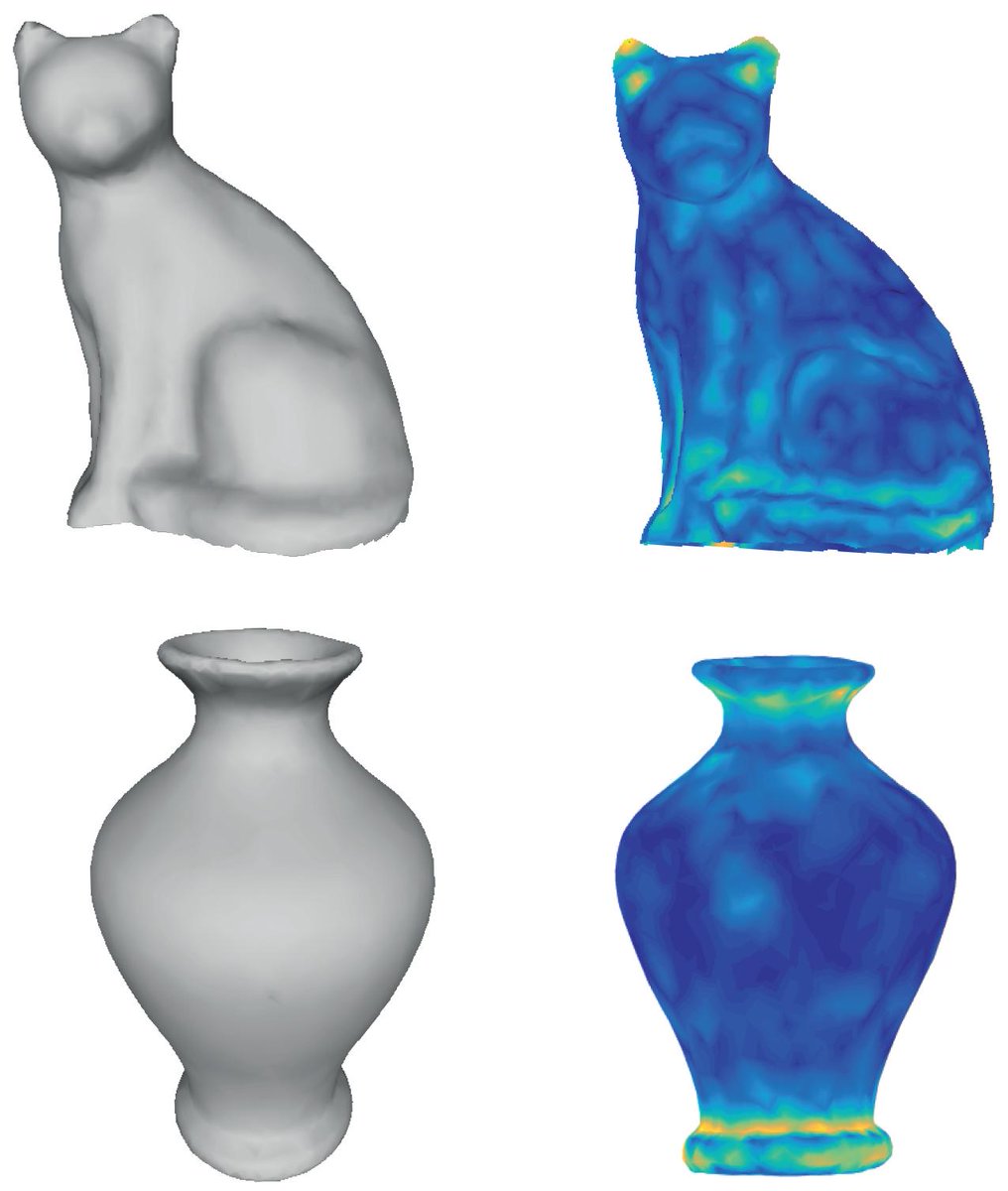
#mdpiinformation New Paper: "Blind Robust 3D Mesh Watermarking Based on Mesh Saliency and Wavelet Transform for Copyright Protection" mdpi.com/413830 @MDPIOpenAccess #3D #watermarking #MeshSaliency #WaveletTransform #QuantizationIndexModulation

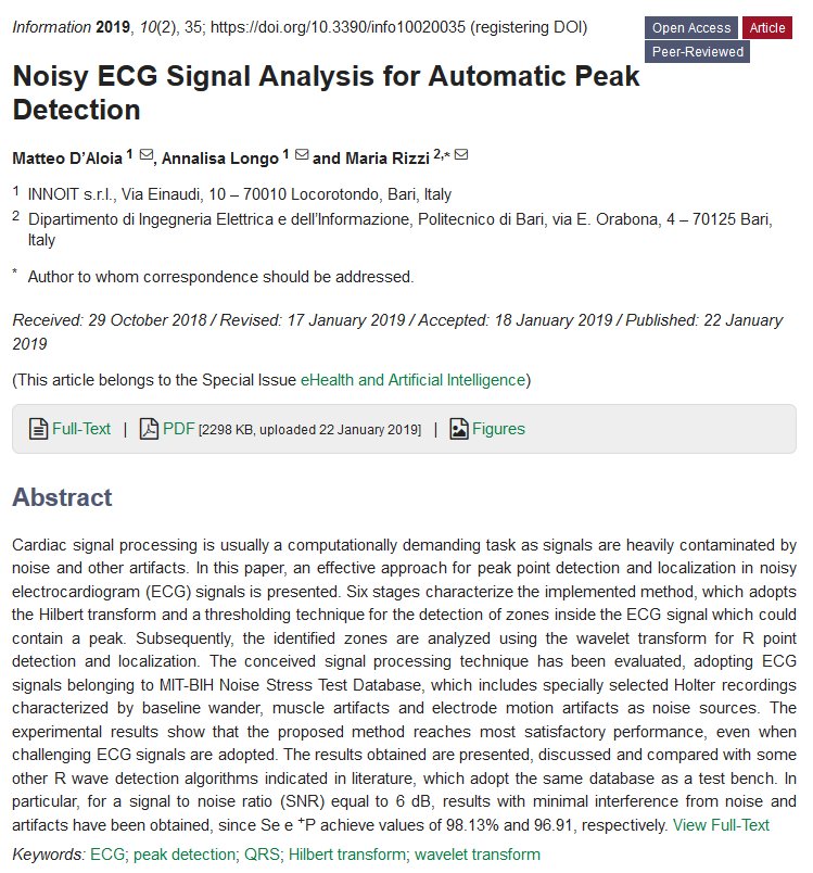
#mdpiinformation Noisy ECG Signal Analysis for Automatic Peak Detection mdpi.com/399516 @MDPIOpenAccess #ECG #PeakDetection #QRS #HilbertTransform #WaveletTransform