
May 26
🎓 Fully Funded PhD in Biostochastics (Sweden 🇸🇪)
💶 Fully funded 4-year PhD with competitive doctoral salary progression outstanding research environment and benefits
✅ Passionate about #ComputationalBiology #DeepLearning #BayesianStatistics 🧬🧠📊
✅ Highly recommend this advanced interdisciplinary #fullyfunded #PhDPosition within the Department of Microbiology, Tumor and Cell Biology at @karolinskainst 🇸🇪
📌 This #phdproject focuses on developing flexible yet interpretable statistical and deep learning models for complex biological systems
You’ll work on:
🔷 Developing new modeling frameworks that bridge mechanistic and data-driven approaches
🔷 Designing and implementing deep learning and generative modeling methods for biological systems
🔷 Working across ecology, phylogenetics, and protein generative modeling applications
🔷 Applying advanced Bayesian inference, stochastic processes, Gaussian Processes, and latent-variable models
🔷 Conducting computational experiments and collaborating with experimental biology labs
🔷 Publishing cutting-edge interdisciplinary research at the intersection of statistics, AI, and biology
🌍 Contribute to next-generation computational biology by developing interpretable and scalable models that advance understanding of complex living systems.
✅ Work with Dr. @BenjMurrell and the Biostochastics research environment at Karolinska Institutet
⏰ 𝗗𝗲𝗮𝗱𝗹𝗶𝗻𝗲: 𝟭𝟱𝘁𝗵 𝗝𝘂𝗻𝗲, 𝟮𝟬𝟮𝟲
👉 Full details & apply here:
🔗 phdscanner.com/opportunities…
📩 Want more like this?
➕ Follow @PhdScanner and join WhatsApp for updates:
whatsapp.com/channel/0029Vb5…
🌐 Visit: phdscanner.com
#fullyfundedPhD #PhDposition #KarolinskaInstitutet #Sweden #Biostochastics #ComputationalBiology #DeepLearning #GenerativeModels #BayesianStatistics #MachineLearning #Bioinformatics #ResearchOpportunity
@phdhardtalk
♻️ Share with someone applying this cycle

ALT https://www.phdscanner.com/opportunities/phd-vacancies-karolinska-institutet-sweden-doctoral-phd-student-position-in-biostochastics-78dffa25-3399-4ad9-94e9-11b4e62a55ef
1
10
546

May 19
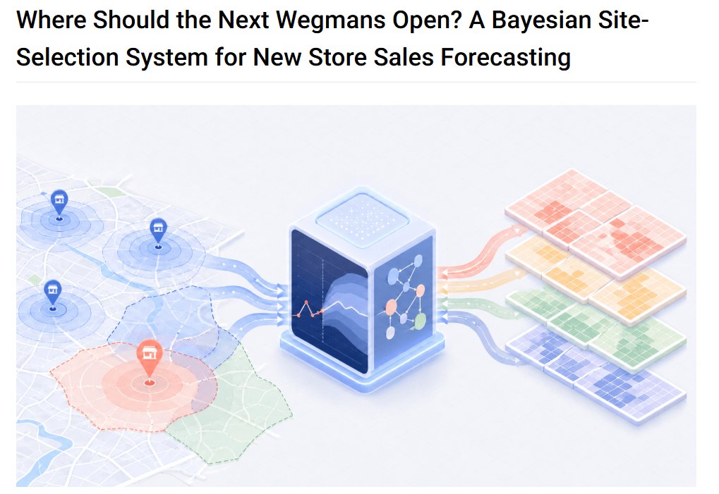
@Wegmans needed to quantify cannibalization risk before opening new stores. We built a Bayesian system that answers in minutes, not weeks.
Full technical walkthrough: dub.sh/jPwJrMy
#RetailAnalytics #BayesianStatistics #PyMC
1
3
287
Apr 30
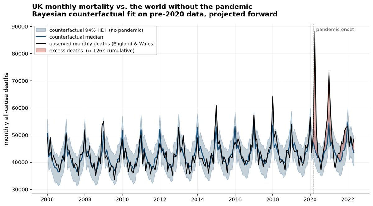
"How many people did COVID kill in the UK?" is the wrong question.
The right one is counterfactual: how many would have died without it?
You can't observe that world. You have to model it.
#BayesianStatistics #PyMC #CausalInference
1
1
8
408

Apr 29
How can Bayesian methods help us learn more from Studies Within A Trial (SWATs)? Find out here where we explore how Bayesian methods and ACCEPT analysis help us get more meaningful insights from SWATs: link.springer.com/article/10… #Trials #TrialMethodology #SWAT #BayesianStatistics
1
3
303

Apr 27
Monte Carlo simulation is a simple but powerful idea: use randomness to approximate values.
A classic example is the value pi. You generate random points inside a square, check whether they fall within a circle, and use the proportion of hits to estimate pi. As the number of samples increases, the estimate becomes more stable and gets closer to the true value.
But there is a limitation. This approach is often presented as a single number, and that number changes every time you run the simulation. So the key question becomes: How uncertain is this estimate at any point in time?
In this setup, each sampled point is either a success or a failure. This allows us to use a Bayesian approach to model uncertainty. Instead of reporting one estimate, we describe a distribution of plausible values for pi given the data and update it as more data is collected.
The visualization below shows this process. On the left, sampled points are added step by step. On the right, the distribution of pi is updated continuously, together with a 95% credible interval. At the beginning, the range of plausible values is wide. As more samples are collected, the distribution becomes narrower and centers around the true value.
This example is based on an article by Pedro Pessoa, who explores this idea in more detail. The graph shown here is also taken from his article: github.com/PessoaP/blog/blob…
In a recent Statistics Globe Hub module, you learn step by step how to design and run Monte Carlo simulations in R, compare statistical methods, and use simulation to answer real research and data science questions.
The Statistics Globe Hub is an ongoing learning program focused on practical skills in statistics, data science, AI, and programming with R and Python.
More info about the Statistics Globe Hub: statisticsglobe.com/hub
#MonteCarlo #BayesianStatistics #DataScience #StatisticalModeling #RStats #Python #MachineLearning #StatisticsGlobeHub
21
124
6,276

NITheCS & SU Dept. of Statistics Seminar:
‘Bayesian study on tumour burden using functional uniform priors in nonlinear mixed-effects models’ by Mia Meyer
📅 Fri, 24 Apr
⏰ 13h10–14h10
🔗 buff.ly/u2fIQeJ
#BayesianStatistics #Biostatistics #NonlinearModels #CancerResearch

2
3
164
Apr 17
Featured case study from the community: a two-pillar Bayesian CLV framework for a nonprofit, built on pymc-marketing.
1M records, MCMC vs. MAP tradeoffs, and a full Databricks deployment walkthrough
Read the blog here: dub.link/jn62Xs9
#PyMC #BayesianStatistics #CLV
1
3
211
Apr 15
University of Amsterdam | PhD in Bayesian Cognitive Modeling & Psychology 🧠📊
🚨 Deadline: May 3, 2026
Join University of Amsterdam 🇳🇱 for a cutting-edge PhD at the intersection of cognitive science, psychology, and Bayesian modeling.
📌 Position: PhD – Bayesian Dynamic Evidence-Accumulation Modeling
🏫 Department: Faculty of Social and Behavioural Sciences
📍 Location: Amsterdam, Netherlands
👨🏫 Supervisor: Dr. Dora Matzke
💰 Salary: €3,059/month (increasing to €3,881)
📆 Duration: 4 years (initial 1 year extension)
🗓️ Start Date: September 2026
💡 Project Focus
Be part of an ERC-funded project exploring how human cognition fluctuates over time using Bayesian models and evidence-accumulation frameworks 📈
🔬 What You’ll Work On
• 🧠 Develop models for cognitive tasks (e.g., Stroop, stop-signal)
• 📊 Build Bayesian hierarchical models linking short- & long-term cognition
• ⏱️ Study variability in human performance across time scales
• 📱 Design large-scale data collection using ecological momentary assessment (EMA)
• 🤝 Collaborate across psychology, math & data science
🌍 Research Impact
• Advance understanding of human cognition & variability
• Improve cognitive testing and predictive models
• Enable real-world applications in health, safety & human performance
• Contribute to next-gen theoretical cognitive frameworks
🎯 Ideal Candidate
• Master’s in Psychological Methods / Cognitive Science / related field
• Experience with Bayesian modeling & response time analysis
• Strong programming skills (R preferred)
• Interest in mathematical psychology & interdisciplinary research
• Good communication & teamwork skills
🎁 Why Apply?
• 💰 Competitive salary bonuses (holiday year-end)
• 🌍 Work in a top European research environment
• 📚 Access to training, conferences & international collaborations
• 🤝 Join a leading lab in mathematical psychology
• 📈 Strong career development opportunities
🌆 Why Amsterdam?
A vibrant, international city known for its research excellence, culture, and high quality of life 🚲
🔗 More Info
phdscanner.com/opportunities…
#PhD #CognitiveScience #BayesianStatistics #Psychology #DataScience #Netherlands #UniversityOfAmsterdam #ResearchJobs #PhDOpportunity
1
3
299
Apr 1
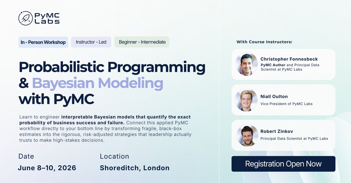
We're bringing Bayesian modeling to London, live and in person!
June 8-10: Learn to build probabilistic models in #PyMC, guided by its creators.
Small cohort, hands-on, walk out with working code. Seats are limited.
👉 dub.link/qWV6KHA
#BayesianStatistics
3
5
429

Consciousness is not a mystery to be narrated.
It is a dynamical regime under constraint.
In META(t), consciousness emerges when two structural conditions are jointly satisfied:
• Information coherence exceeds a bifurcation threshold
• Available energy exceeds a physical minimum (Landauer-bound derived)
This yields four falsifiable predictions:
1. Non-linear bifurcation
2. Necessary information–energy coupling
3. Quantified structural residue
4. Strict dissociation between activation and expression
If any fails, the model self-invalidates.
Preprint (ResearchGate):
DOI: 10.13140/RG.2.2.29371.48165
@grok ton avis?
#Consciousness #Neuroscience #CognitiveScience #ComputationalNeuroscience #ComplexSystems #InformationTheory #Thermodynamics #Falsifiability #BayesianStatistics #AI
@ResearchGate: researchgate.net/publication…
2
12

Feb 17
Glad to contribute to this important Bayesian analysis of FINEARTS-HF evaluating Finerenone in HFmrEF/HFpEF.
Using robust meta-analytic predictive priors informed by FIDELIO-DKD, FIGARO-DKD, and TOPCAT, Bayesian modeling confirmed and strengthened the frequentist signal:
• Primary outcome (CV death total HF events): RR 0.83 (95% CrI 0.74–0.94)
• ≥10% relative risk reduction: posterior probability ↑ from 90% → 92% with informative priors
• CV death: 80% probability of benefit (HR 0.93; CrI 0.79–1.10)
• All-cause mortality: 85% probability of benefit (HR 0.94; CrI 0.83–1.06)
As expected, hyperkalaemia risk increased, with reduced hypokalaemia.
#HFpEF #HFmrEF #Finerenone #MRA #CardioTwitter #BayesianStatistics #HeartFailure #EvidenceBasedMedicine
Bayesian analysis of finerenone in heart failure with mildly reduced and preserved ejection fraction: a pre-specified analysis of FINEARTS-HF academic.oup.com/ehjcvp/arti…
2
6
22
2,039

Python for data science and statistical computing in PhD research.
Taught by Mark Andrews, Senior Lecturer in Psychology and long standing instructor in applied Bayesian data analysis.
7–8 April
prstats.org/course/python-fo…
#PhDStudents #Python #DataScience #BayesianStatistics

3
27

24 Nov 2025
6
234

6 Oct 2025
📣 Deal of the Day 📣 Oct 6
HALF OFF NEW MEAP!
Grokking Bayes & selected titles: hubs.la/Q03Mqf-b0
A complete guide to thinking in Bayes, full of fun illustrations and friendly introductions. @the_subtrahend #Bayesian #BayesianStatistics #BayesianInference #ProbabilisticProgramming #PyMC #stats #statistics
Bayesian statistics is a framework for reasoning under uncertainty. You'll first build an intuition, and then translate that intuition into working code with Python tools like the PyMC library and ArviZ package. Along the way, you'll explore how Bayesian ideas connect to modern AI, from uncertainty-aware deep learning to LLM applications.

1
1
5
813

10 Sep 2025
The use of Bayesian methods in the design of trials and the analysis of the findings provides several potential benefits, which may be particularly applicable in Trauma & Orthopaedic surgery.
#ClinicalTrials #BayesianStatistics #RCTs #Ortho @docfarrow
ow.ly/xeXm50WRwZN
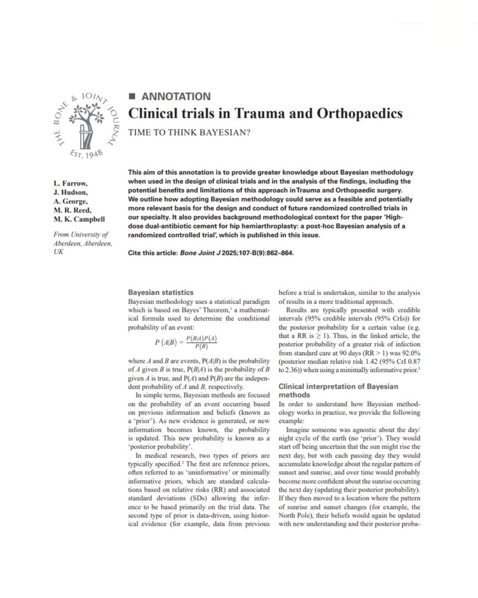
ALT The Bone & Joint Journal. Extract from article titled 'Clinical trials in Trauma and Orthopaedics: time to think Bayesian?'
3
6
895

9 Sep 2025
Out Now! Learning ecosystem-scale dynamics from microbiome data with MDSINE2 bit.ly/3K0yguN #Microbiome #BayesianStatistics #EcosystemDynamics

1
48
127
9,752

2 Sep 2025
Last week, I wrapped up my time as a Visiting Researcher @UniTurku. Grateful to @antagomir, his team, and many Finnish colleagues for a summer that was both scientifically enriching 🔬 and personally memorable 😍. Excited about the new projects we’re starting together 🚀 and future collaborations ahead 🤝! #Statistics #Biostatistics #Microbiome #Multiomics #DataScience #MultimodalAI #MachineLearning #BayesianStatistics

3
83

11 Aug 2025
This is a great little book by @profpauldolan .
Just to have the concept of #beliefism more in the national consciousness would be an advantage to all of us.
But it should also be taught at schools, along with other vital concepts currently missing from a desperately tired national curriculum, like #socialcontagion #bayesianstatistics, etc.

2
4
551
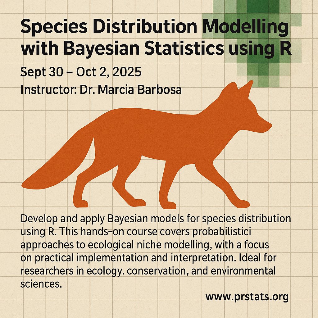
Online Course - Live and Online
Registration:
prstats.org/course/online-co…
#SpeciesDistributionModelling #BayesianStatistics
#EcologicalModelling #RStats #QuantitativeEcology
#SpatialEcology #EnvironmentalDataScience
#Biostatistics #EcologyTraining #StatisticalModelling
2
5
99

11 May 2025
Bayesian variable selection stochastic search in R 🔍
Check out this great ML-ready guide by Lukasz Gatarek 👉 blog.devgenius.io/bayesian-v…
#rstats #DataScience #MachineLearning #BayesianStatistics #RProgramming
4
43
3,730